Synopsis

MR Fingerprinting (MRF) can simultaneously map multiple parameters and can be used to compute estimates of tissue fractions. However, MRF-derived M₀ maps contain information about both proton density (PD) and the receiver sensitivity profile (RP). Here we estimate relative PD and RP from MRF M₀ and T₁ maps. Relative PD and tissue fractions are combined for absolute quantity mapping of CSF, gray matter, and white matter as a fraction of the voxel equilibrium magnetization.

Introduction

Background

MRF-derived M₀ maps contain information about both PD and the receiver sensitivity profile (RP). We express the MRF-M₀ map as the product of the PD and RP.

Measuring RP is challenging, particularly at higher fields. To overcome this issue, we propose using a previously described relationship between T₁ and PD in white matter (WM) and gray matter (GM) [9]:

Eq1 $$\frac{1}{PD}\approx A + \frac{B}{T_1}$$

where A and B are constants. Because RP does not affect quantitative MRF T₁ maps, we propose using the T₁ map to form an estimate of PD, which can then be used with the MRF M₀ map to estimate RP.

Methods

Volunteers were scanned with FISP-MRF [2] at 3T (Skyra, Siemens Healthcare, Erlangen, Germany). To evaluate the technique for different receiver profiles, the same acquisition was performed with a 20-channel head coil and the body coil. MRF parameters were as follows: TR_min 8.64ms, maximum flip angle 30°, 3000 frames, FOV 300mm, resolution 1.17x1.17x5mm. Voxelwise dictionary matching was based on the inner product [1].

T₁ and T₂ values corresponding to pure GM, WM, and CSF, and partial volumes were identified by 7-component k-means analysis. Clusters identifying pure WM, pure GM, and WM/GM partial volumes were included in a mask for PD fitting. MRF tissue fraction maps for WM, GM, and CSF were estimated using a dictionary-based approach [4].

MRF PD maps and the receiver profile were estimated from the normalized M₀ map as described by Volz et al [10]. A pure CSF voxel was chosen as an internal PD reference and the M₀ map was normalized to this signal. A pseudo PD map was initialized based on Eq1, taking constants A & B from literature [10] and T₁ values from within the GM/WM mask. The RP was approximated inside the mask from M₀ and pseudo PD after Gaussian filtering, then fit to a 2^nd order 2D polynomial and extrapolated across the whole brain. An estimate of PD was made across the whole brain, normalized to CSF, then used to estimate constants A & B within the GM/WM mask. The process was repeated until A & B stabilized.

Absolute tissue maps were created by voxelwise multiplication of the tissue fractions with the normalized PD. ROIs 7mmx7mm were placed bilaterally in various brain structures for quantitative comparisons.

Results

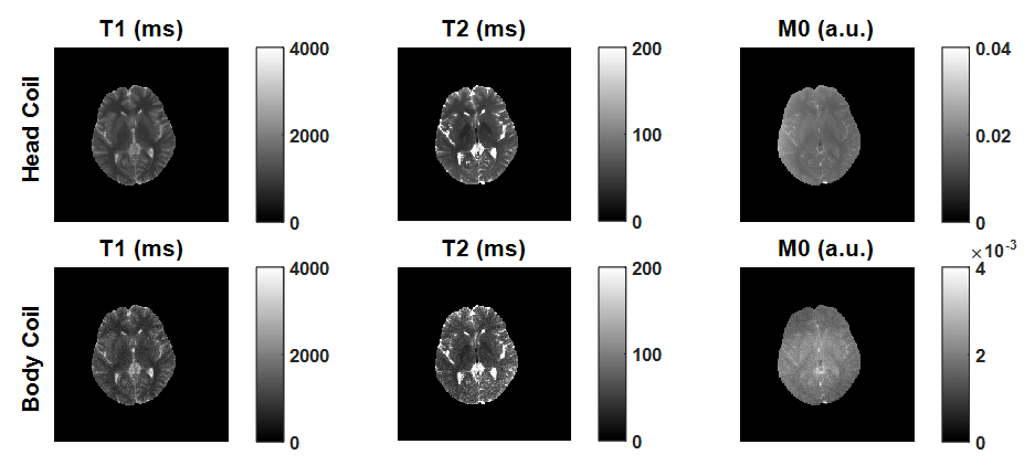
Figure 1 shows MRF maps measured from head and body coils. The M₀ maps illustrate the effect of different receive profiles.

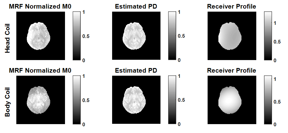
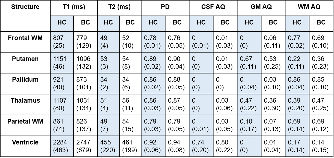
Figure 2 shows the MRF M₀ map, and the estimated PD and RP after 7 iterations. The mean PD values are in very close agreement across structures (Table 1). Fitted constants for Eq2 were A_HC=0.788, B_HC=395ms in the head coil, and A_BC=0.824, B_BC=352ms in the body coil.

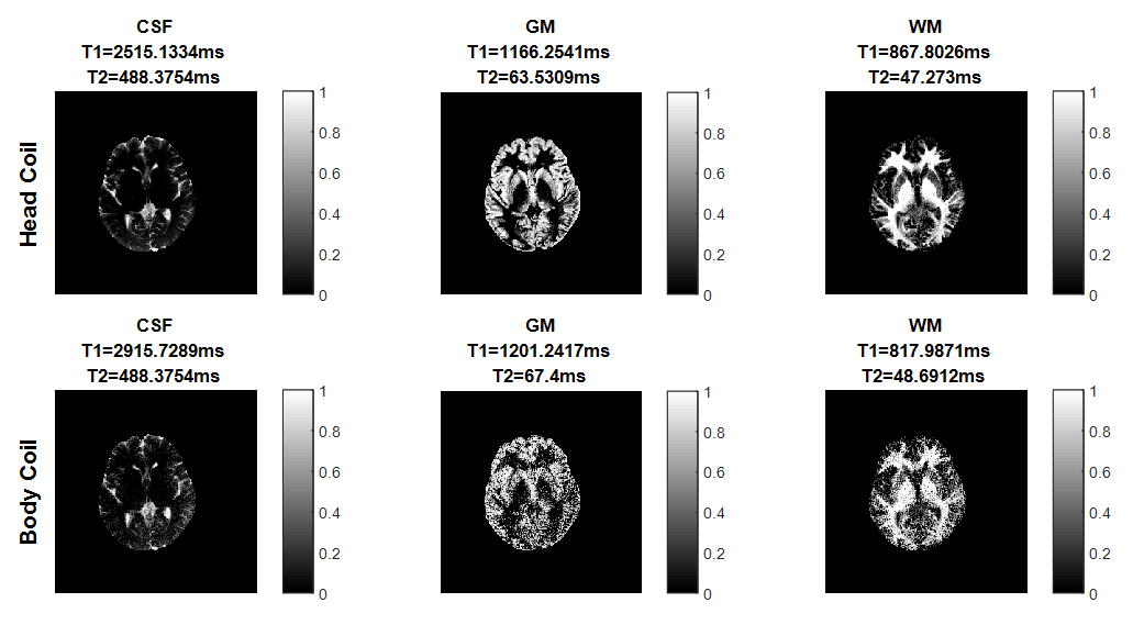
Figure 3 shows tissue fraction maps for CSF, GM, and WM. T₁ and T₂ values of each tissue type in the PV analysis differ by 5% or less between the two acquisitions, even given the noisy body coil results.

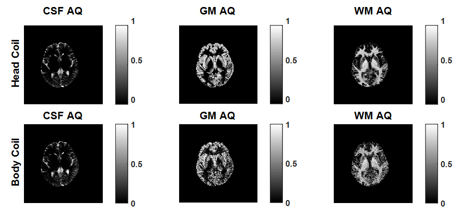
Figure 4 shows absolute quantity maps for CSF, GM, and WM as a fraction of the equilibrium magnetization. Absolute quantities in each ROI are shown in Table 1.

Conclusions

We demonstrated the ability to estimate PD and receiver profile directly from MRF, which can also be used to generate quantitative maps of T₁, T₂, and tissue fractions. Estimated PD maps are in good agreement in multiple acquisitions, demonstrating robust separation of different receiver profile effects. This approach could have implications beyond MRF, potentially providing high quality B₁- maps at high field strengths. In this experiment we could combine the PD and tissue fraction maps to quantify the relative contribution of each tissue type to the voxel magnetization.

The PD and RP estimation presented here uses a global fitting approach. More accurate PD and RP estimates may be obtained through multi-channel fitting [11]. B₁+ mapping may further improve the accuracy of these maps.

Acknowledgements

References

[1] Ma et al. Magnetic Resonance Fingerprinting. Nature 2013; 495(7440):187-192.

[2] Jiang et al. MR Fingerprinting using Fast Imaging with Steady State Precession (FISP) with Spiral Readout. Magnetic Resonance in Medicine 2015; 74(6):1621-1631.

[3] Deshmane et al. Validation of Tissue Characterization in Mixed Voxels Using MR Fingerprinting. Proc. ISMRM 2014; p.94.

[4] Deshmane et al. Enforcing a Physical Tissue Model for Partial Volume MR Fingerprinting. Proc. ISMRM 2016; p.2998.

[5] McGivney et al. The Partial Volume Problem from a Bayesian Perspective. Proc. ISMRM 2016; p.435.

[6] Tofts. Quantitative MRI of the Brain: Measuring Changes Caused by Disease. 2003; John Wiley & Sons, Ltd.

[7] Laule et al. Water Content and Myelin Water Fraction in Multiple Sclerosis: A T2 Relaxation Study. J Neurology 2004; 251(3):284-293.

[8] Shah et al. Quantitative Cerebral Water Content Mapping in Hepatic Encephalopathy. NeuroImage 2008; 41(3):706-717.

[9] Fatouros et al. In Vivo Brain Water Determination by T1 Measurements: Effect of Total Water Content, Hydration Fraction, and Field Strength. Magnetic Resonance in Medicine 1991; 17(2) 402-413.

[10] Volz et al. Quantitative Proton Density Mapping: Correcting the Receiver Sensitivity Bias via Pseudo Proton Densities. NeuroImage 2012; 63: 540-552.

[11] Mezer et al. Evaluating Quantitative Proton-Density-Mapping Methods. Human Brain Mapping 2016; 37(10):3623-3635.