1350
Quality Factors for Efficient and Precise MRF Imaging1Physics, Case Western Reserve University, Cleveland, OH, United States, 2Biomedical Engineering, Case Western Reserve University, Cleveland, OH, United States, 3Radiology, University Hospitals Case Medical Center, Cleveland, OH, United States
Synopsis
With the invention of MRF imaging, there is considerable freedom in input parameter selection, but it is difficult to determine how each choice affects the resulting parameter maps. Quality factors are introduced as a means of comparing MRF sequences with various input parameters (FA, TR, TE, N) on their abilities to precisely quantify T1 and T2. Simulations, fully sampled, and undersampled experiments verified that sequences with higher quality factors result in lower standard deviations in R1 and R2. With quality factor analysis, researchers and clinicians can readily determine the appropriate MRF input parameters to image more efficiently and precisely.
Purpose
To introduce a means of analysis by which the efficacy of various MRF sequences can be judged. The desire for quantitative MRI has led to the recent introduction of MRF, which allows for simultaneous multi-parametric quantization of imaging parameters including relaxation times T1 and T2 [1]. However, it has been shown that the precision of parameter quantification depends on the chosen imaging sequence parameters, including FA, TR, TE, and number N of repetitions (steps) [2]. In this work, we introduce quality factors that can be used to determine the precision with which an imaging sequence can quantify T1 and T2 relaxation times. The results were verified in simulation and experiments with both fully sampled and undersampled data.Methods
The goal of this work is to develop a mathematical framework with which the error in measuring relaxation times using various MRF sequences can be quantitatively assessed. MRF experiments can then be performed with assurance that chosen imaging parameters (FA, TR, TE, and N) will successfully produce reliable T1 and T2 maps.
The standard deviations of R1=1/T1 and R2=1/T2 are related to the dictionary signals through a multivariate Taylor series expansion of transverse magnetization about $$$R1_0$$$ and $$$R2_0$$$ at each time step. Then the first order corrections to the N-dimensional dictionary vector $$$\overrightarrow{D_{0}}=\overrightarrow{D}\left(R1_0,R2_0\right)$$$ yield $$\overrightarrow{D}\left(R1,R2\right)\cong\overrightarrow{D_{0}}+\overrightarrow{C1}\left(R1-R1_0\right)+\overrightarrow{C2}\left(R2-R2_0\right)$$ with N-dimensional coefficients $$$\overrightarrow{C1}$$$ and $$$\overrightarrow{C2}$$$, containing the first derivative of the transverse magnetization with respect to R1 and R2 respectively at each time step. Thus, the acquired signal with noise $$$\eta$$$ from a tissue with $$$R1_{0}$$$ and $$$R2_{0}$$$ will be $$$\overrightarrow{S}=\overrightarrow{D_0}+\overrightarrow{\eta}$$$.
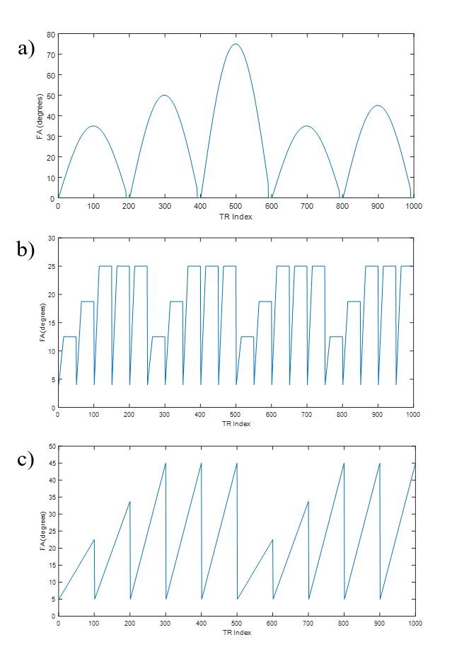
The extremum calculation of the dot product $$$Re\left(\overrightarrow{S}\cdot\overrightarrow{D}^*\right)$$$ leads to the standard deviations $$$\sigma_{R1}=\frac{\eta}{\sqrt{Q1}}$$$ and $$$\sigma_{R2}=\frac{\eta}{\sqrt{Q2}}$$$ with quality factors $$Q1=C1^{2}\frac{1+2\;\widehat{D_{0}}\cdot\widehat{C2}^{\star}\;\widehat{D_{0}}\cdot\widehat{C1}^{\star}\;\widehat{C1}\cdot\widehat{C2}^{\star}-\left(\widehat{D_{0}}\cdot\widehat{C2}^{\star}\right)^{2}-\left(\widehat{D_{0}}\cdot\widehat{C1}^{\star}\right)^{2}-\left(\widehat{C1}\cdot\widehat{C2}^{\star}\right)^{2}}{1-\widehat{D_{0}}\cdot\widehat{C2}^{\star}}$$ and $$Q2=C2^{2}\frac{1+2\;\widehat{D_{0}}\cdot\widehat{C2}^{\star}\;\widehat{D_{0}}\cdot\widehat{C1}^{\star}\;\widehat{C1}\cdot\widehat{C2}^{\star}-\left(\widehat{D_{0}}\cdot\widehat{C2}^{\star}\right)^{2}-\left(\widehat{D_{0}}\cdot\widehat{C1}^{\star}\right)^{2}-\left(\widehat{C1}\cdot\widehat{C2}^{\star}\right)^{2}}{1-\widehat{D_{0}}\cdot\widehat{C1}^{\star}}$$ where all individual products are understood to be $$$Re\left(\overrightarrow{A}\cdot\overrightarrow{B}^\star\right)$$$, and $$$\overrightarrow{C1}$$$ and $$$\overrightarrow{C2}$$$ are obtained through first order parametric fitting.The quality factors were initially tested with Bloch equation simulations in MATLAB, where error analysis was performed by repeatedly matching a simulated signal containing Gaussian white noise to a pre-calculated dictionary by maximizing $$$Re\left(\overrightarrow{S}\cdot\overrightarrow{D}^*\right)$$$. The matching was repeated for various FAs, TRs, TEs, Ns, and preparation pulses for both FISP-based and bSSFP-based MRF sequences [3][4]. A FISP-MRF experiment was then performed (3T Siemens Skyra and an 18-channel brain array coil) with a variable-density spiral (48 projections for full k-space coverage, 192x192, 300mm2 FOV) and a phantom with ten separate compartments each with a different T1 and T2 combination. Three FA distributions of 1000 steps were tested (see figure 1) with TE=0.75ms and TR=6.98ms [3][4]. Matching for N=1000 and N=500 produced T1 and T2 maps from the fully sampled data, from which the standard deviations of matched R1 and R2 were calculated for each gel. Finally, matching was performed over 1000 and 500 steps to produce T1 and T2 maps for the FA distributions in Figure 1, with undersampled experimental data (acceleration factor R=48).
Results
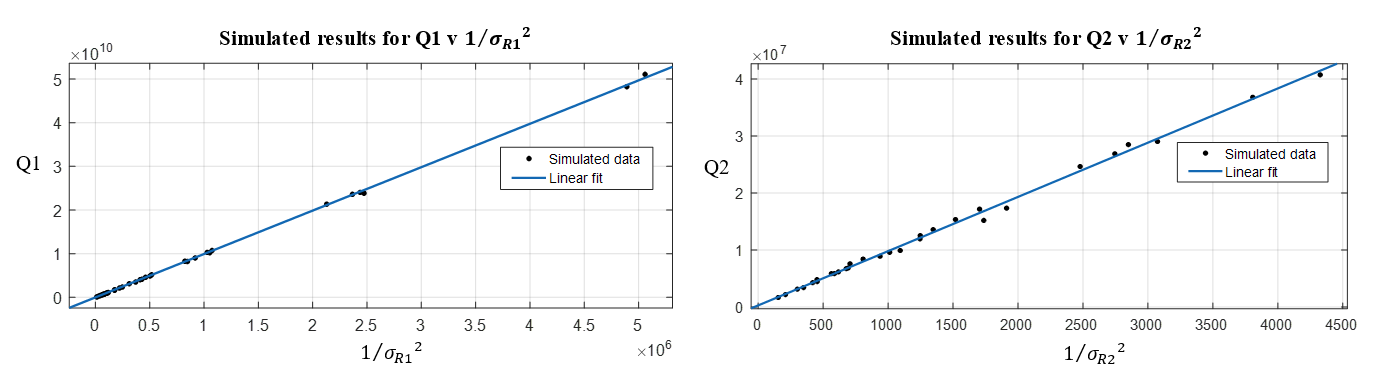
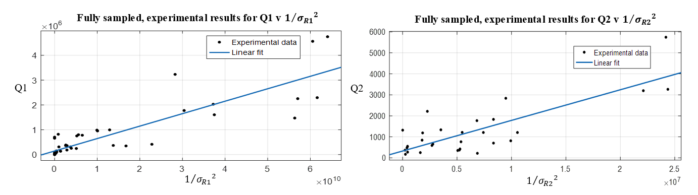
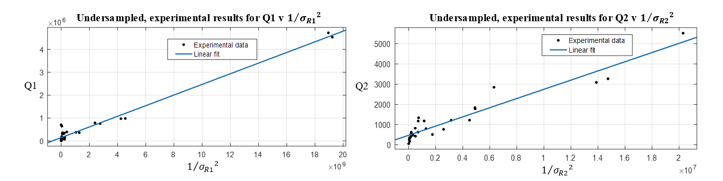
The results of matching simulated and experimental data to a dictionary are presented for six values of T1 and T2 with ranges [370, 1710] ms and [40,105] ms respectively. Shown in Figure 2, simulated results demonstrate exemplary linearity between Q1 and 1/$$$\left(\sigma_R1 \right)^2$$$ and Q2 and 1/$$$\left(\sigma_R1 \right)^2$$$, where $$$\sigma_R1$$$, and $$$\sigma_R2$$$ were calculated by matching simulated noisy data to the dictionary. Figure 3 shows the results of matching the fully sampled, experimental data and Figure 4 shows result of matching the undersampled, experimental data. The fully sampled data contains significant scatter from the expected linear result, likely due to local and non-additive experimental uncertainties, which is overwhelmed by global and additive undersampling noise resulting in improved linearity in analysis the undersampled experimental data.
Discussion
The results of simulated, fully sampled experimental, and undersampled experimental MRF matching show that Q1 and Q2 successfully gauge the error with which a given MRF experiment can measure T1 and T2. Specifically, Q1 and Q2 can predict how changing the number of imaging steps taken, and changing the TR, TE, and FA distributions can improve or worsen the ability of the experiment to precisely match T1 and T2.Conclusion
Through simulation and experiment, we find that the larger Q1 and Q2 are, the smaller standard errors in R1 and R2 will be. With the utilization of quality factors it is possible for researchers and clinicians to determine the effectiveness of a given set of FA, TR, and TE distributions over N steps to match T1 and T2; additionally, quality factor analysis can act as a springboard for optimization of input imaging parameters thus allowing them to image more quickly and precisely.Acknowledgements
NIH T32EB007509. OTF IPP TECG20140138.References
[1] Ma D, et al. Nature 495, 187-92 (2013). [2] Hamilton J et al. Proc. ISMRM 2015:3386. [3] Jiang Y, et al. MRM 74:1621–1631 (2015). [4] Hamilton J et al. MRM doi:10.1002/mrm.26216.Figures