1317
Analytic description of the magnetisation phase during excitation1Dept. Electrical and Computer Systems Engineering, Monash Institute of Medical Engineering, Monash University, Clayton, Australia, 2Monash Biomedical Imaging, Monash University, Clayton, Australia, 3Faculty of Medicine, Department of Neurology, JARA, RWTH Aachen University, Aachen, Germany
Synopsis
An approximate analytic expression is calculated for the phase of the transverse magnetisation during the excitation period. A spherical Bloch equation is used to find this expression. Simulation results are in agreement with the analytic solution. This analytic solution can be used where the phase information is required and, therefore, may be used to improve the performance of imaging through optimal pulse sequence design.
Introduction
Finding analytic expressions to describe the behaviour of the magnetisation vector for different types of pulses has attained considerable attention in the Magnetic Resonance (MR) literature1-4. In this paper, we provide an approximate analytic expression to describe the phase of the transverse component of the magnetisation vector during excitation that can be used for optimal designing of pulse sequences in Magnetic Resonance Imaging (MRI) . We have validated the analytic solution by comparing it to the numerical solution of the Bloch equation. Simulation results demonstrate that the analytic expression follows the numeric solution with an acceptable level of error for tip angles up to $$$\pi/2$$$ for all isochromats.Methods
Assuming the Radio Frequency (RF) field is applied in the x'-direction, the Bloch equation during excitation for short pulses in the spherical coordinates for azimuth and colatitude components of the magnetisation vector in the rotating frame of reference can be written as5
$$ \left\{ \begin{array}{l l} \dot{\theta} = -\Delta \omega_0+\omega_1(t) \cot \phi \cos \theta\\ \dot{\phi} = \omega_1(t) \sin\theta\\ \end{array} \right.$$
where $$$\Delta \omega_0$$$ is the filed inhomogeneities including gradient fields, $$$\omega_1(t) $$$ is the excitation field, $$$\theta = \tan^{-1}\frac{M_{y'}}{M_{x'}}$$$ and $$$\phi = \cos^{-1}M_{z'}$$$ in which $$$M_{x'}$$$, $$$M_{y'}$$$ and $$$M_{z'}$$$ are the magnetisation components in the Cartesian coordinates. We have used available tools in nonlinear dynamical systems6,7 to find the phase of the magnetisation as follows
$$\theta (t) \approx \frac{\pi}{2} - \Delta\omega_0\,t +\tan^{-1}\left(\cot\int_0^t\omega_1(\tau) \cos(\Delta\omega_0\tau)\, d\tau \,\,\tanh \int_0^t\omega_1(\tau) \sin(\Delta\omega_0 \tau)\,d\tau \right).$$
The above expression is valid for hard as well as soft RF pulse excitations. Furthermore, if field inhomogeneities are time varying, e.g. time varying gradient fields, the above equation applies by replacing $$$\Delta\omega_0 \tau$$$ with $$$\int_0^\tau \Delta\omega_0(s) ds$$$.
Simulation Results
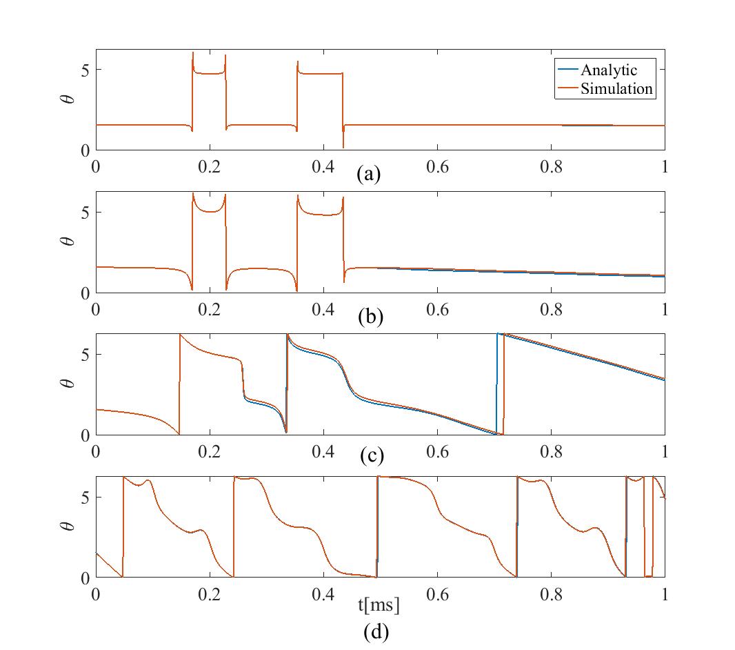
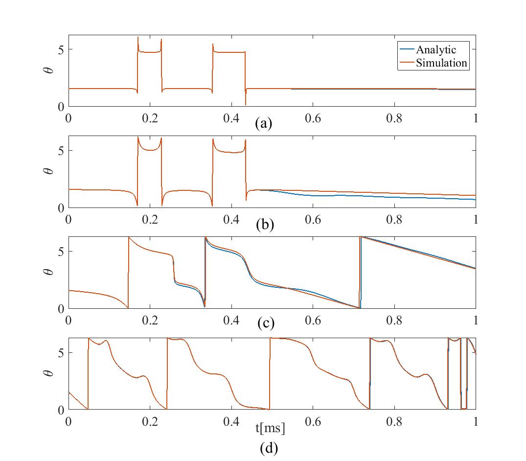
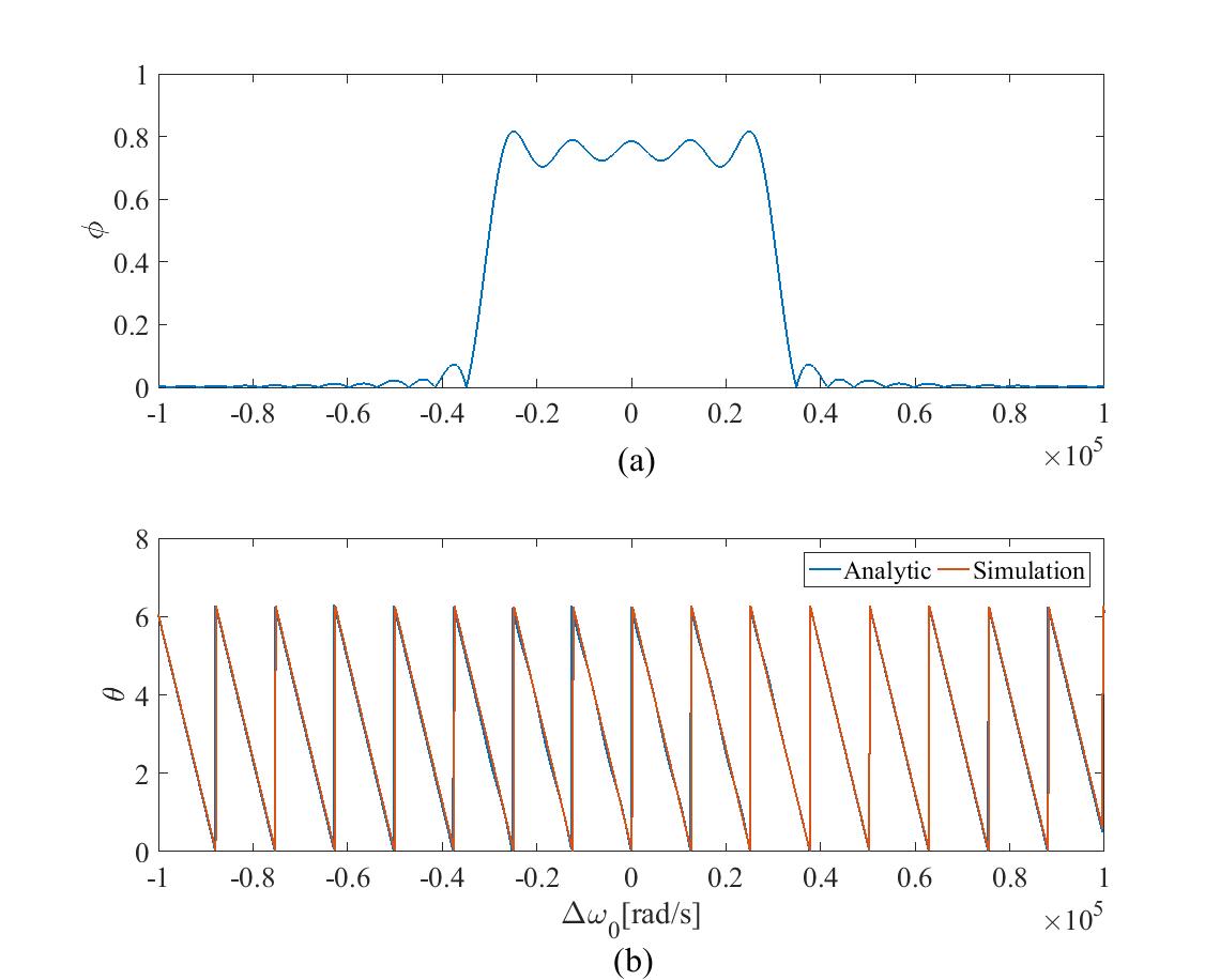
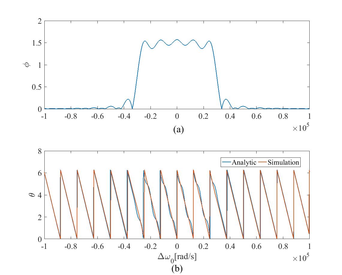
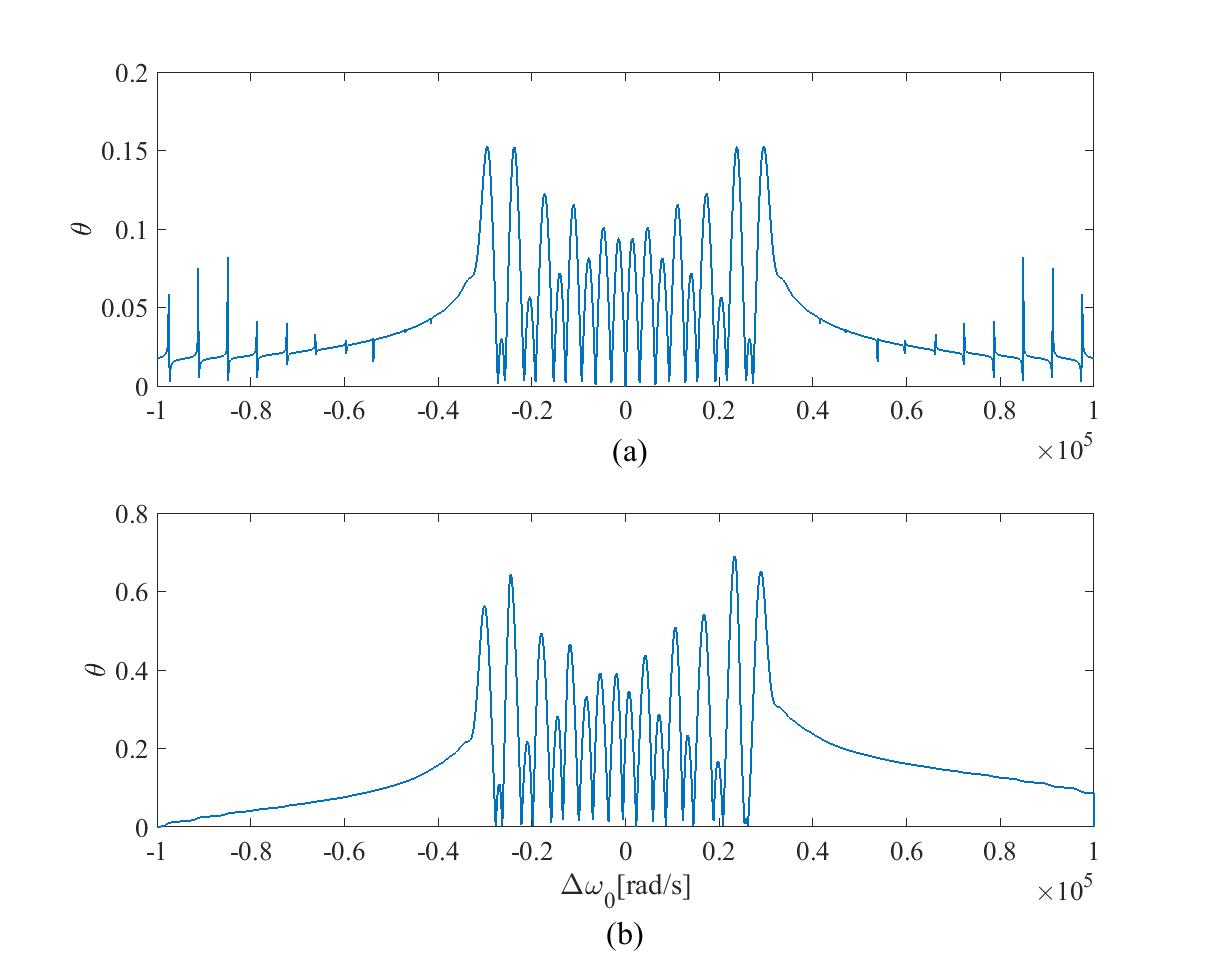
To investigate the validity of the approximate analytic solution, we have compared the numerical solution of the Bloch equation using ode45 in MATLAB to the analytic expression for $$$\theta$$$ provided in the Methods section. Figure 1 represents the analytic and numeric solution to the Bloch equation for a $$$\pi/4$$$ slice selective sinc pulse with 1ms duration. The results for four isochromats are illustrated in this figure. Figure 2 shows the results for a $$$\pi/2$$$ slice selective pulse. These results demonstrate how the analytic solution tracks the numerical results. Figures 3 and 4 represent the simulation result of the Bloch equation for $$$\pi/4$$$ and $$$\pi/2$$$ selective pulses, respectively. These simulations show the discrepancy between the analytic and numeric solution is more pronounced inside the slice. The error between the analytic and numeric solution for both pulses is depicted in Figure 5. The maximum error for the $$$\pi/4$$$ pulse is about 15% while for the $$$\pi/2$$$ pulse, the error increases to 38%.Conclusion
An analytic expression that describes the phase of the transverse magnetisation vector during excitation was presented. Numerical simulations of the Bloch equation are in agreement with the analytic expression. This solution can be used to estimate the phase of the magnetisation at the end of the pulse and, therefore, can be used to improve the performance of pulse sequences where the phase of the transverse component is important, e.g. phase imaging8-10 or for short and zero echo time imaging11. Furthermore, it is possible to estimate a more accurate tip angle using the analytic phase expression and the spherical Bloch equation.Acknowledgements
No acknowledgement found.References
1. D.I. Holt, "The solution of the Bloch equations in the presence of a varying B1 field - An approach to selective pulse analysis," Journal of Magnetic Resonance, vol. 35, pp. 69-86, 1979.
2. J. Pauly, D. Nishimura, and A. Macovski, "A k-space analysis of small tip-angle excitation," Journal of Magnetic Resonance, vol. 81, pp. 43-56, 1989.
3. N. Boulant and D.I.Hoult, "High Tip Angle Approximation Based on a Modified Bloch-Riccati Equation," Magnetic Resonance in Medicine, vol. 67, pp. 339-343, 2012.
4. J. Zhang, M. Garwood, and J.Y. Park, "Full Analytical Solution of the Bloch Equation when Using a Hyperbolic-Secant Driving Function," Magnetic Resonance in Medicine, DOI: 10.1002/mrm.26252, 2016.
5. B. Tahayori, L.A. Johnston, I.M.Y. Mareels, and P.M. Farrell, "Novel insight into magnetic resonance through a spherical coordinate framework for the Bloch equation," in Proceedings of the SPIE Conference on Medical Imaging, Physics of Medical Imaging, pp. 72580Y1-72580Y12, Orlando, USA, Feb. 2009.
6. J. Sanders, F. Verhulst, and J. Murdock, Averaging Methods in Nonlinear Dynamical Systems. Springer-Verlag, 2007.
7. H. Khalil, Nonlinear Systems, 3rd ed. Prentice Hall, 2002
8. K. Shmueli , J.A.de Zwart, P. van Gelderen , T.Q. Li, S.J. Dodd, J.H. Duyn, "Magnetic susceptibility mapping of brain tissue in vivo using MRI phase data," Magnetic Resonance in Medicine, vol. 62, pp. 1510–1522, 2009.
9. E.M. Haacke, S. Liu, S. Buch, W. Zheng, D. Wu, and Y. Ye, "Quantitative susceptibility mapping: current status and future directions," Magnetic Resonance Imaging, vol. 33, pp. 1–25, 2015.
10. S.D. Robinson, B. Dymerska, W. Bogner, M. Barth, O. Zaric, S. Goluch, G. Grabner, X. Deligianni, O. Bieri, and S. Trattnig, "Combining phase images from array coils using a short echo time reference scan (COMPOSER)," Magnetic Resonance Imaging, DOI: 10.1002/mrm.26093, 2015.
11. M. Garwood, "MRI of fast-relaxing spins," Journal of Magnetic Resonance, vol. 229, pp. 49-54, 2013.
Figures