1266
Tridimensional Axial and Circumferential WSS from 4D flow data using a finite element method and a Laplacian approach1Biomedical Imaging Center, Pontificia Universidad Católica de Chile, Santiago, Chile, 2Department of Electrical Engineering, Pontificia Universidad Católica de Chile, Santiago, Chile, 3Department of Radiology, School of Medicine, Pontificia Universidad Católica de Chile, Santiago, Chile, 4Department of Biomedical Engineering, King's College London, London, United Kingdom, 5Department of Structural and Geotechnical Engineering, Pontificia Universidad Católica de Chile, Santiago, Chile
Synopsis
The WSS and OSI play a critical role in the progression of different vascular diseases, the multidirectional nature of WSS, can alter the balance of the endothelial cells. But the multidirectional nature of WSS only has been analyzed in 2D section. In this work, we propose a new method based on 3D finite-element and a Laplacian approach to decompose the WSS vector in an axial (WSSA) and circumferential (WSSC) component in a 3D domain. The 3D method provides an excellent agreement of the quantification of WSSA and WSSC in comparison with the actual 2D method.
Purpose
There is evidence that the non-uniform wall shear stress (WSS) and oscillatory shear index (OSI) play a critical role in the progression of different vascular diseases1,2. Previously proposed 2D WSS methods allow evaluating this multidirectional nature of WSS in patients, decomposing the WSS vector in an axial (WSSA) and circumferential (WSSC) components. Previous studies have found that the circumferential WSS is a significant parameter to be analyzed in patient with BAV and atherosclerosis3,4,5.
Recently, a few methods have been proposed to obtain the WSS in a 3D domain6,7, however the magnitude of WSS does not allow the analysis WSSA and WSSC independently. The reason for this limitation is that for the 3D methods a reference plane is not available as it is for the 2D methods. One exception is the use of centerlines in 3D domain8 to generate reference planes for each node of the surface of the vessel of interest. However, the use of centerlines in complex geometries can induce errors to calculate 2D planes perpendicular to the vessel of interest. In this work, we propose a novel method based on 3D finite-element and a Laplacian approach to decompose the WSS vector in an axial and circumferential component in a 3D domain, that can be used in any geometry.
Methods
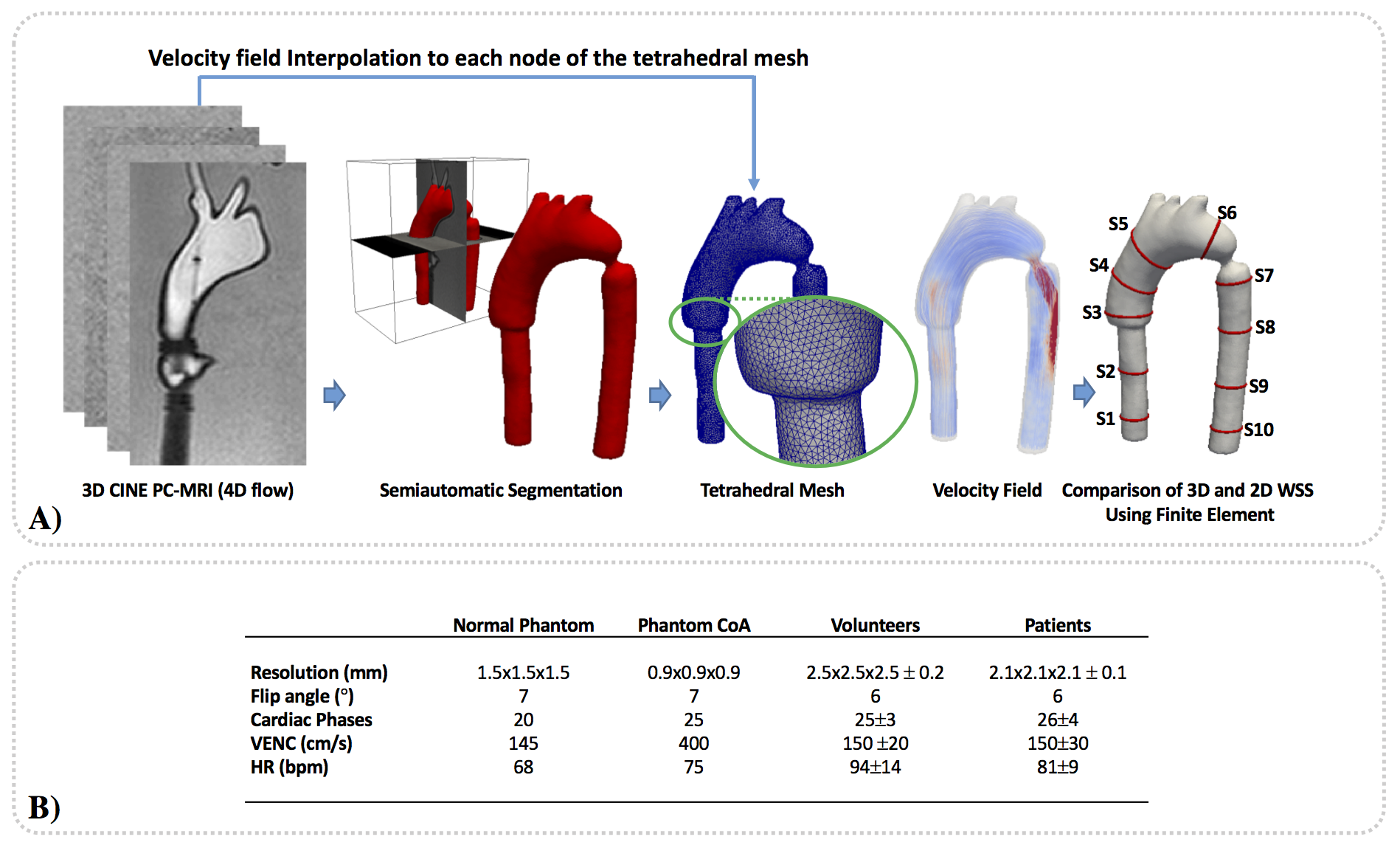
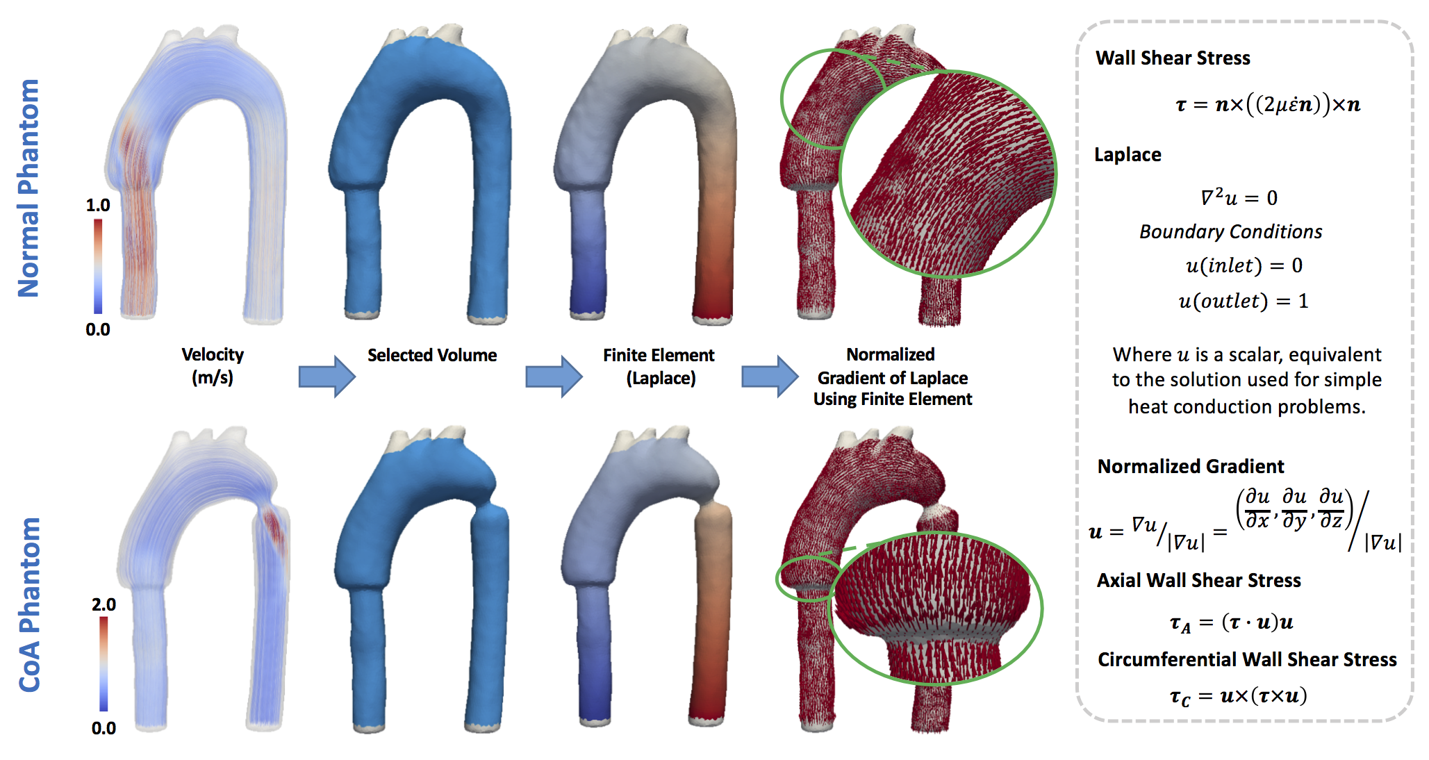
Using a MR Philips Achieva 1.5T, we acquired 4D-flow data set of one realistic aortic phantom, to validate our method9. The phantom was acquired in normal conditions (normal phantom) and with an aortic coarctation (CoA phantom) of 9mm. The proposed quantification process of the phatom data is described in figure1. To create the tetrahedral finite-element mesh we use the available toolbox iso2mesh for Matlab. Ten different sections were created to compare the WSSA and WSSC proposed by our 3D method and a previously published 2D method, also based on finite-elements10. Using these sections, we analyzed the differences between both methods using Bland-Altman plots and Wilcoxon signed rank test (p≤0.05 was considered statistical significant). The WSS vector in 3D domain was calculated using a finite-element method previously published7. To decompose the WSS vector in WSSA and WSSC components, we compute a finite-element formulation based on the Laplace equation, with two dirichlet boundary condition at the inlet and outlet face (see figure2). Then, a normalized gradient was calculated over the solution of Laplace to generate axial normal vectors in each node of the 3D domain. Finally using these axial normal vectors, we calculated the WSSA and WSSC components from the 3D WSS solution7. The finite-element analysis was developed using the Python software. For the visualization and analysis of the data we used the open source software Paraview. To show the applicability of our method we analyzed 4D flow data of the aorta of six healthy children (four females and two males, age 14.7±5.1 years) and seven Fontan children patients (two females and five males, age 10.7±2.1 years). The acquisition MR parameters used to acquire in-vitro and in-vivo data is shown in figure1.Result
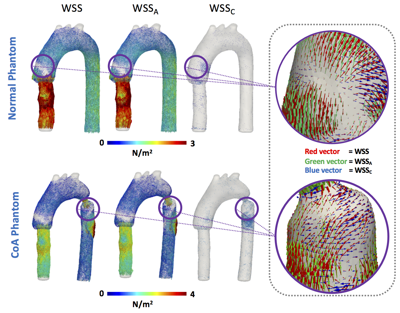
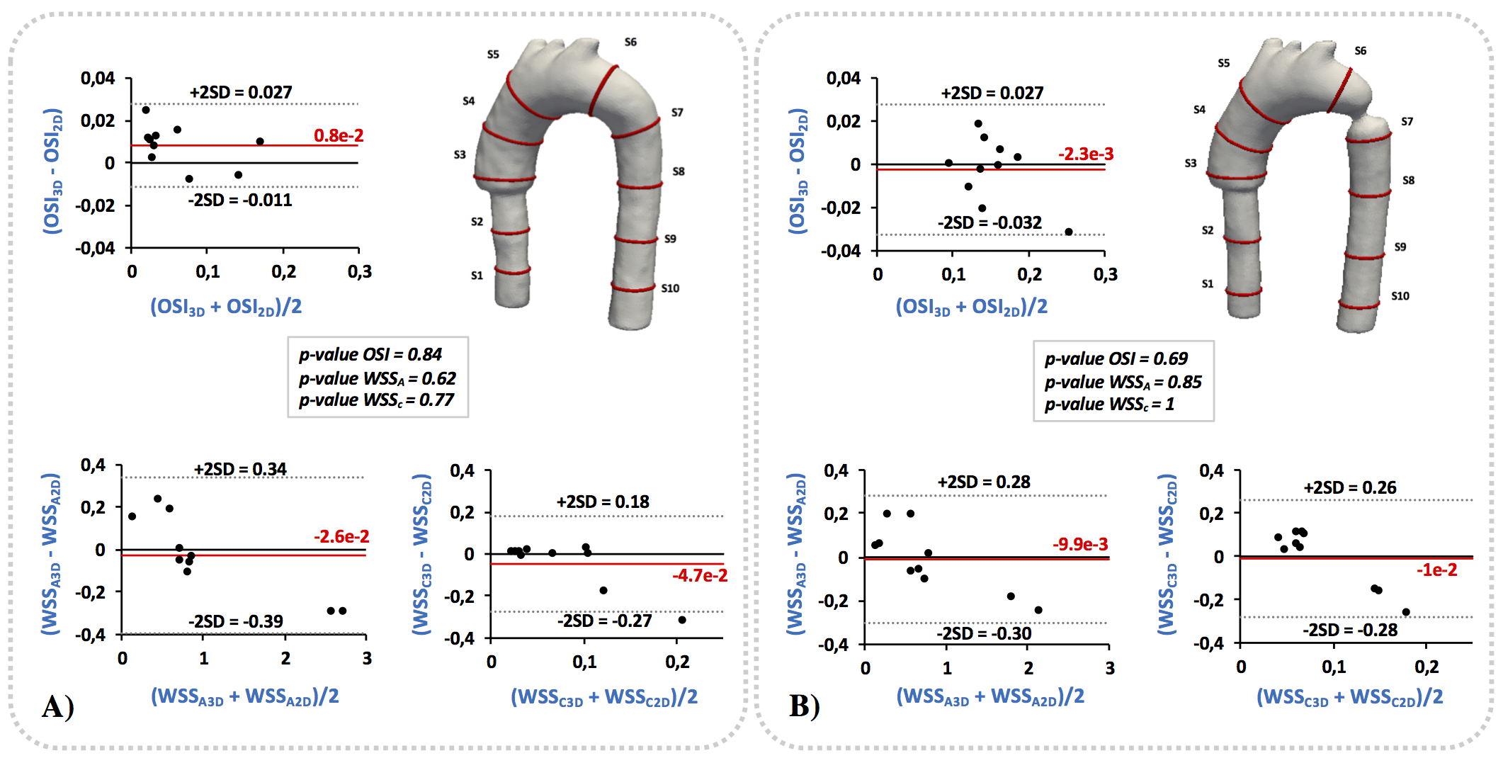
The distribution of WSS, WSSA and WSSC vectors for the normal phantom and the CoA phantom are shown in figure3. To demonstrate the differences between the WSS components, a color characterization of the WSS, WSSA and WSSC values are presented in figure3. A Bland & Altman comparison of the OSI, WSSA and WSSC contour mean values between the 3D and the 2D method for all section of the normal phantom and CoA phantom is shown in figure4. A negligible bias and not significant differences were observed between both methods for all analyzed parameters.
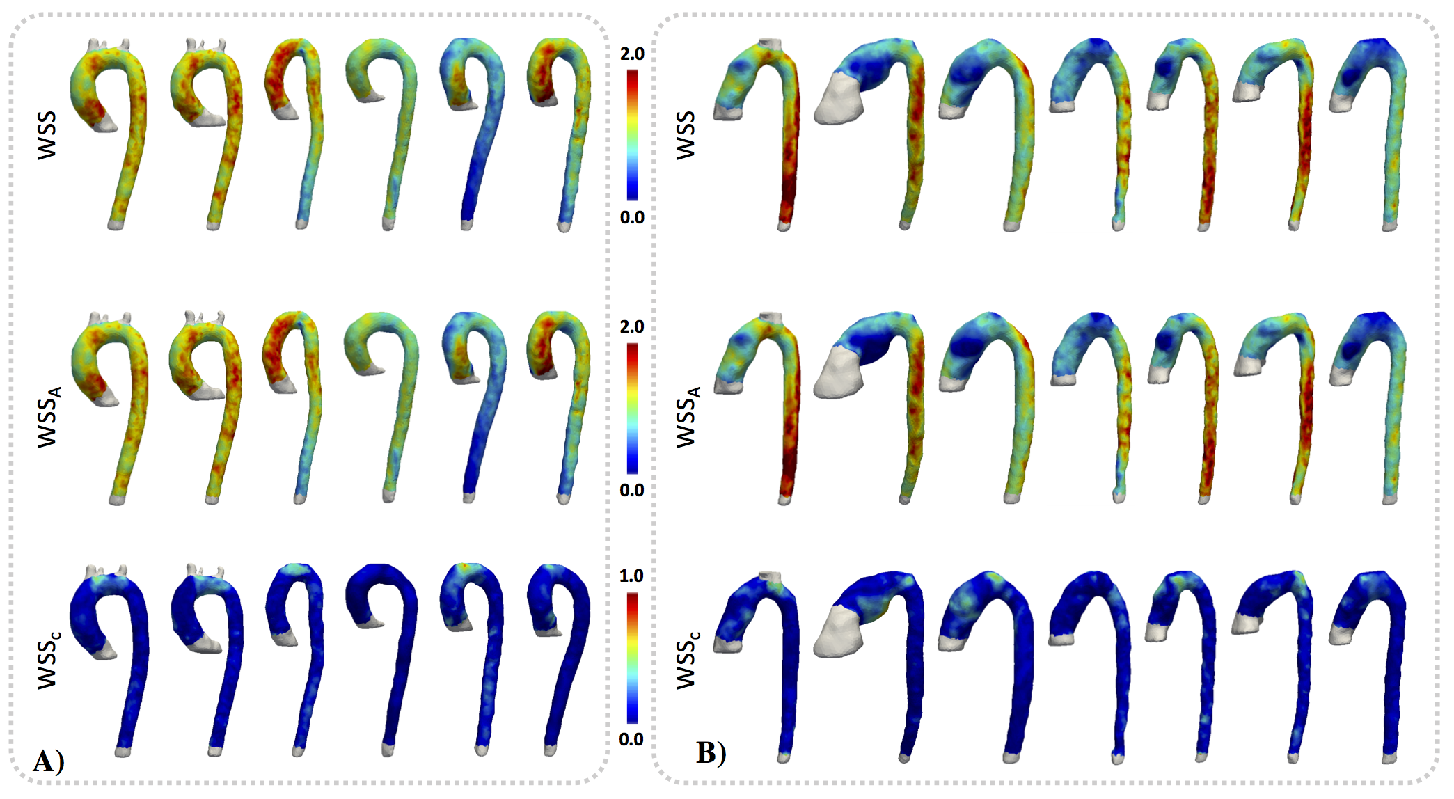
The results of the application of our method in in-vivo data set are shown in figure5. In Fontan patients, we found increased values of WSSC in the ascending aorta in comparison with the group of healthy volunteer. We also found elevated values WSSA in the descending aorta of these patients.
Discussion and Conclusion
We have developed a novel methodology to decompose the 3D WSS vector in WSSA and WSSC components in a 3D domain. The proposed method provides an excellent quantification of WSSA and WSSC in comparison with the actual 2D method. A great advantage of the presented method is that the methodology can be apply to complex geometries as is usually found in patients with cardiovascular diseases. The application of our method in Fontan Patients found significant differences of the WSSC and of the WSSA in the ascending and descending aorta respectively. As future work we will apply our method in patient with BAV where the circumferential WSS has been reported as a relevant biomarker4.Acknowledgements
Thank to grant, CONICYT - PIA - Anillo ACT1416, CONICYT FONDEF/I Concurso IDeA en dos etapas ID15|10284, and FONDECYT #1141036. Sotelo J. Thanks to the School of Engineering, Pontificia Universidad Catolica de Chile, for his Post-Doctoral Fellow.References
1. Traub O, Berk BC. Laminar shear stress: Mechanisms by which endothelial cells transduce an atheroprotective force. Arterioscler Thromb Vasc Biol. 1998 May;18(5):677-85.
2. Wang C, Baker BM, Chen CS, Schwartz MA. Endothelial cell sensing of flow direction. Arterioscler Thromb Vasc Biol. 2013 Sep;33(9):2130-6.
3. Stalder AF, Russe MF, Frydrychowicz A, et al. Quantitative 2D and 3D phase contrast MRI: optimized analysis of blood flow and vessel wall parameters. Magn Reson Med. 2008 Nov;60(5):1218-31.
4. Barker AJ, Lanning C, Shandas R. Quantification of hemodynamic wall shear stress in patients with bicuspid aortic valve using phase-contrast MRI. Ann Biomed Eng. 2010 Mar;38(3):788-800.
5. Mohamied Y, Rowland EM, Bailey EL, et al. Change of direction in the biomechanics of atherosclerosis. Ann Biomed Eng. 2015 Jan;43(1):16-25.
6. Potters WV, van Ooij P, Marquering H, et al. Volumetric arterial wall shear stress calculation based on cine phase contrast MRI. J Magn Reson Imaging. 2015 Feb;41(2):505-16
7. Sotelo J, Urbina J, Valverde I, et al. 3D Quantification of Wall Shear Stress and Oscillatory Shear Index Using a Finite-Element Method in 3D CINE PC-MRI Data of the Thoracic Aorta. IEEE Trans Med Imaging. 2016 Jun;35(6):1475-87.
8. Morbiducci U, Gallo D, Cristofanelli S, et al. A rational approach to defining principal axes of multidirectional wall shear stress in realistic vascular geometries, with application to the study of the influence of helical flow on wall shear stress directionality in aorta. Journal of Biomechanics. Volume 48, Issue 6, 13 April 2015, Pages 899–906.
9. Urbina J, Sotelo JA, Springmüller D, et al. Realistic aortic phantom to study hemodynamics using MRI and cardiac catheterization in normal and aortic coarctation conditions. J Magn Reson Imaging. 2016 Sep;44(3):683-97.
10. Sotelo J, Urbina J, Valverde I, et al. Quantification of wall shear stress using a finite-element method in multidimensional phase-contrast MR data of the thoracic aorta. J Biomech. 2015 Jul 16;48(10):1817-27.
Figures