1263
Compressed Sensing accelerated 4D flow MRI using a pseudo spiral Cartesian sampling technique with random undersampling in time1Department of Radiology, Academic Medical Center, Amsterdam, Netherlands, 2Department of Biomedical Engineering & Physics, Academic Medical Center, Amsterdam, Netherlands
Synopsis
Clinical applications of three-dimensional time-resolved (4D) flow MRI are still hindered by long acquisition times. Using compressed sensing image reconstruction, undersampled 4D flow data may be recovered without a notable loss of image quality. In this study pseudo-spiral sampling on a Cartesian grid was implemented on a Philips 3T Ingenia system to facilitate random undersampling in time. The technique was tested under controlled conditions in a pulsatile phantom for different acceleration factors. An additional in vivo volunteer data set confirmed the stability of this technique.
Introduction
4D flow MRI involves a trade-off between acquisition time, spatiotemporal resolution, and signal-to-noise ratio (SNR). Compressed sensing (CS) is an emerging reconstruction technique, that requires randomly undersampled data and can facilitate a reduction of acquisition time1,2. Previous implementations of 4D Cartesian undersampling strategies showed promising results3,4. Since total variation (TV) in time serves as a good sparsifying transform for 4D flow data, random undersampling over time was implemented on a 3T Philips system. Sampling profiles (ky,kz) were continuously changed during each cardiac cycle and retrospectively binned, which resulted in a different undersampling pattern per time frame. A pseudo spiral Cartesian sampling scheme was applied to avoid high eddy currents. This technique was validated using acceleration factors up to 10X for a pulsatile flow phantom and 6X for a volunteer scan.
Methods
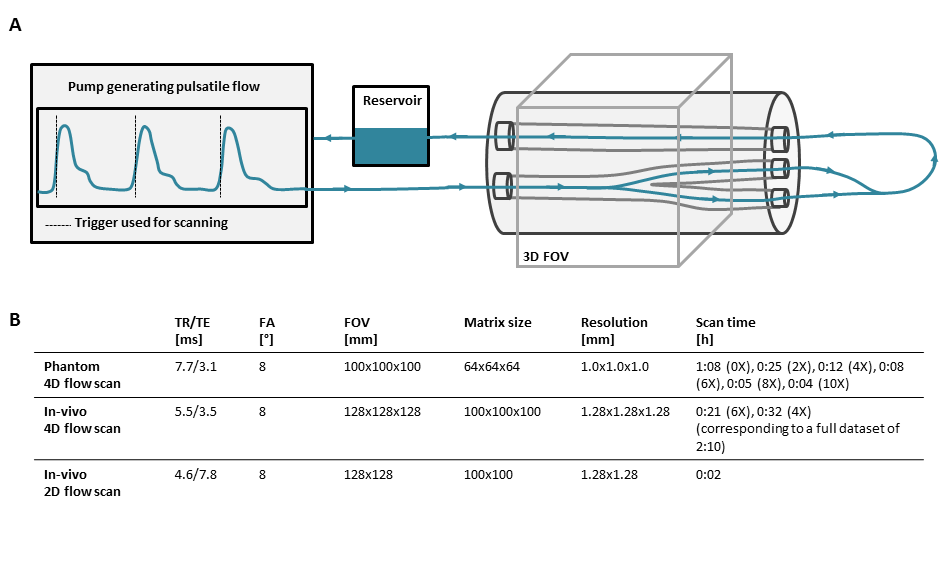
4D flow measurements were performed on a carotid bifurcation phantom (LifeTec, Eindhoven, Netherlands). A pulsating water flow with a simulated heart rate of 60 bpm and a variability of 5% created a temporal mean flow of 300 ml/min. A timestamp from the pump signal was used for retrospective triggering. A schematic overview of the experimental setup and all measurement parameters are shown in Figure 1. All experiments were conducted on a 3T MRI scanner (Philips Healthcare, Best, Netherlands) using an 8-channel neck coil. The volunteer was a 26 year old male with no history of cardiovascular disease.
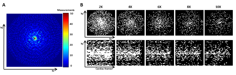
The scanner software was modified to acquire a predefined number of sampling profiles. The sampling profiles (ky,kz) were generated with MATLAB (The MathWorks Inc., Natick, MA, USA) as points of multiple spiral trajectories with variable density gridded on a matrix of size 64x64 (Figure 2A). The number of sampling profiles was calculated based on the desired undersampling factor and number of cardiac phases. During each heartbeat (ky,kz) profiles were consecutively changed. With this sampling strategy and a physiological heart rate variability, retrospective binning according to trigger time created a unique sampling pattern per cardiac frame (Figure 2B). A total matrix size of 64x64x64 was acquired in three flow encoding directions using a VENC of 150 cm/s. Profile lists of different lengths were created with a nominal acceleration factor of 2X, 4X, 6X, 8X, and 10X; whereby the in vivo experiment only used 4X and 6X acceleration. The acquired data was processed by ReconFrame (Gyrotools, Zurich, CH) and retrospectively absolute binned, selecting 24 cardiac frames. CS reconstruction was performed using Berkeley Advanced Reconstruction Toolbox (BART)5 with a sparsifying TV transform in time and a wavelet transform in space (x,y,z) and time. The L1-regularisation was performed with a regularisation parameter of r = 0.01 and 50 iteration steps.
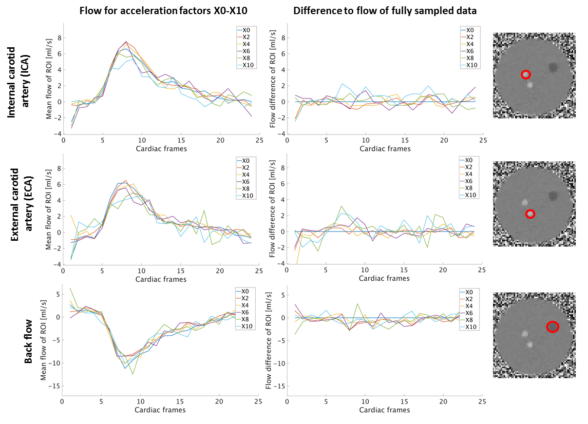
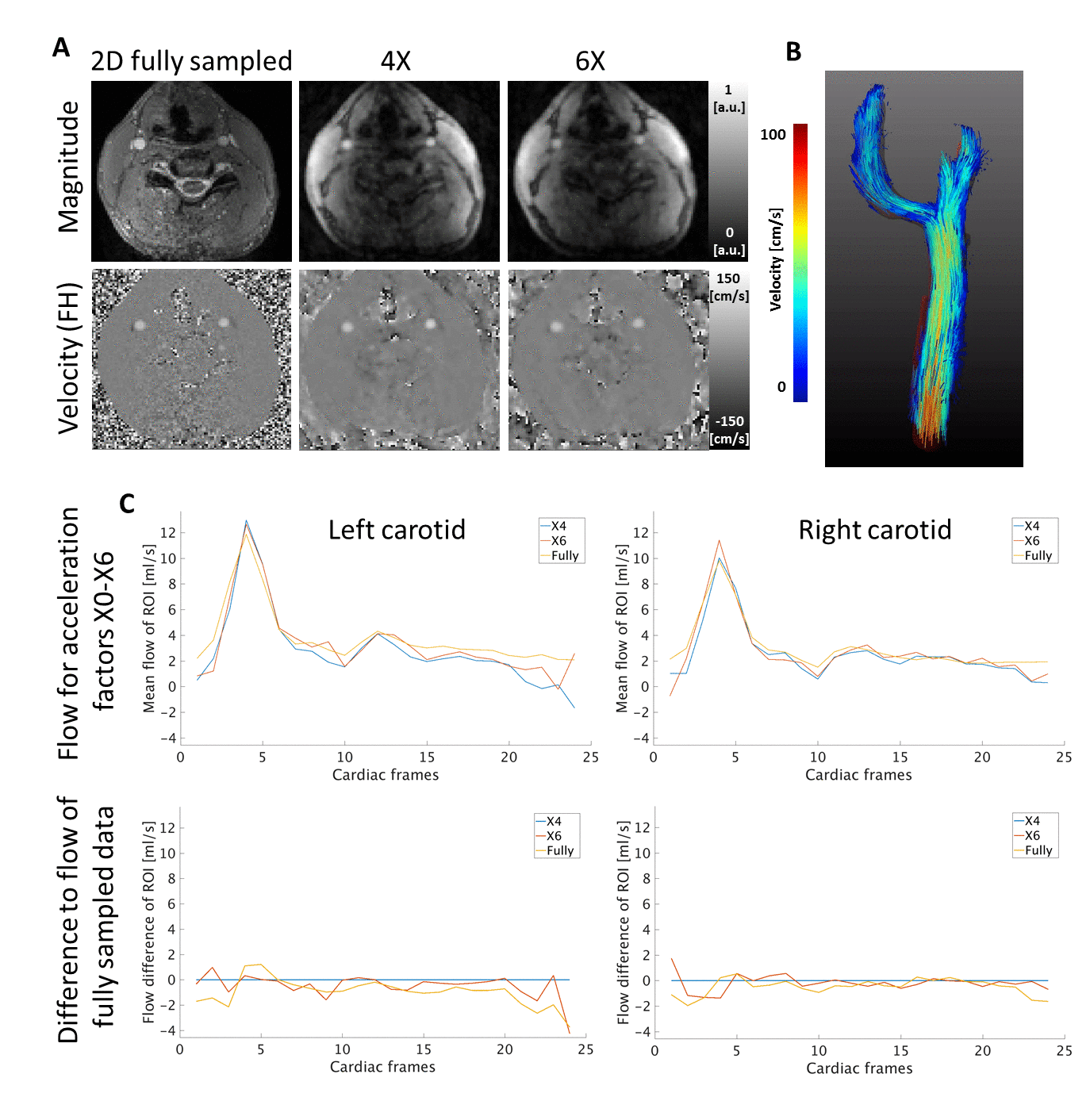
For the phantom experiment, a non-accelerated scan was performed for both voxel-by-voxel comparisons with the accelerated scans (difference images) and comparison of flow curves averaged over the vessel region. The accelerated volunteer scan was compared to a fully sampled 2D data set, and flow curves together with streamline visualizations were evaluated.
Results
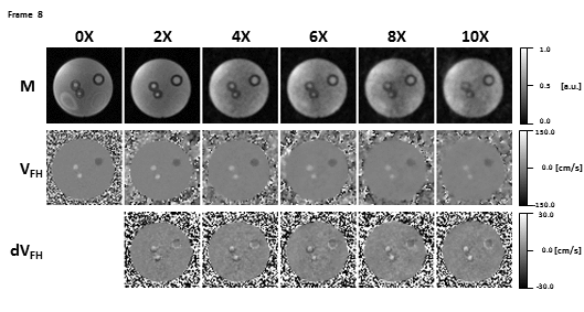
Taking both the unique sampling pattern for each of the 24 cardiac frames and the arrhythmia rejection into account, the actual mean undersampling factors over all frames were 3.39$$$\pm$$$0.48X, 5.55$$$\pm$$$0.92X, 7.75$$$\pm$$$1.29X, 9.88$$$\pm$$$1.57X, and 12.12$$$\pm$$$2.23X. Figure 3 shows magnitude, velocity, and velocity difference images of undersampled data in comparison to the fully sampled data. Velocity difference images show deviations up to 20% (10X). Flow curves for all measurements are shown in Figure 4. The flow differences of the accelerated data range from 0.35ml/s to 2.66ml/s at the main systolic peak. Figure 5 shows results of a 4X and 6X accelerated 4D flow data set in a healthy volunteer compared to the same slice acquired in a fully sampled 2D acquisition. It can be seen that the difference between the curves ranges from 1% (4X) to 5% (6X).Discussion
Starting from an acceleration factor of 6X the image quality decreases. Similarly, flow curves show minor deviations up to an acceleration factor of 6X. The in vivo measurements demonstrated acceptable performance at an acceleration factor of 6X and agreed well with the time-resolved 2D scan at high spatiotemporal resolution.Conclusion
We have successfully implemented a variable density pseudo-spiral Cartesian sampling strategy of consecutively changed (ky,kz) profiles during each cardiac cycle. In combination with a physiological heart rate variability and retrospective binning, data acquisition resulted in a unique undersampling pattern per cardiac frame. A CS reconstruction could recover data by exploiting sparsity under TV transform in time. A significant decrease in scan time up to a factor of 6X could be achieved while maintaining acceptable image quality and accurate flow estimations.Acknowledgements
N/AReferences
1. Lustig, Michael, et al., “Compressed Sensing MRI.” Signal processing Magazine 2008; Vol. 72:1053-5888.
2. Lustig, Michael, et al., “Sparse MRI: The application of compressed sensing for rapid MR imaging.” Magn. Reson. Med. 2007; Vol. 58:1182-1195.
3. Wetzl, Jens, et al. "Free-Breathing, Self-Navigated Isotropic 3-D CINE Imaging of the Whole Heart Using Cartesian Sampling." Proc. Intl. Soc. Mag. Reson. Med. 2016; Vol. 24.
4. Cheng, Joseph Y., et al. "Variable-density radial view-ordering and sampling for time-optimized 3D Cartesian imaging." Proceedings of the ISMRM Workshop on Data Sampling and Image Reconstruction 2013, Sedona, Arizona, USA.
5. Uecker, Martin, et al. "Berkeley advanced reconstruction toolbox." Proc. Intl. Soc. Mag. Reson. Med. 2015; Vol. 23.
Figures