Synopsis

MRSI can benefit greatly from ultra-high field strengths. Given the higher SNR and higher chemical shift dispersion, metabolite mapping can be done with higher quantification precision and at higher spatial resolution. The aim of this work was to study the competing effects of spatial resolution, SNR, linewidth and higher field strengths by pushing the spatial resolution limits of 3T and 9.4T for metabolite mapping of the human brain.

Introduction

It has previously been shown that MRSI can benefit greatly from ultra-high field strengths^1-3. Given the higher SNR and higher chemical shift dispersion, metabolite mapping can be done with higher quantification precision and at higher spatial resolution. However, due to long scan times associated with higher resolution scans, higher spectral line-widths due to technical difficulties such as B₀ and B₁ inhomogeneity at higher field strengths, the advantages with respect to metabolite mapping might not be as great as one expects.

The aim of this work was to study the competing effects of spatial resolution, SNR, linewidth and higher field strengths by pushing the spatial resolution limits of 3T and 9.4T for metabolite mapping of the human brain.

Methods

A total of 6 healthy volunteers were scanned, 4 at 9.4T and 2 at 3T. The studies were performed on a 9.4T Siemens whole-body human scanner (Erlangen, Germany) using a 16Tx/31Rx in-house developed coil⁴ and on a 3T Siemens Prisma scanner using a commercial 64 channel head and neck coil. A single-slice FID MRSI sequence with an optimized 3 pulse water suppression scheme was used with slice thickness of 10mm and FOV of 200x200mm. Parameters for 3T and 9.4T were, respectively: flip angle = 55/28; bandwidth = 2400/8000Hz, acquisition time = 425/128ms; TR=550/220ms, Acquisition delay=2.1/1.5ms.

The studies were done at increasingly higher spatial resolution on each volunteer, as long as the scan time was acceptable. For each volunteer, acquisitions were done both fully sampled and accelerated in two separate sessions. Acceleration was done using a 2x2 GRAPPA⁵ with 6 auto-calibration lines.

At 9.4T, this allowed scanning of spatial resolutions of 32x32, 64x64, 128x128 and 160x160, and at 3T, spatial resolutions of 32x32 and 64x64.

All spectra were processed using a custom software written in MATLAB. Post processing steps included eddy current and zero-phase correction using a non-water suppressed reference image acquired at 2x2 times lower spatial resolution, SVD coil combination⁶, removal of the water residual using HLSVD method⁷, and automatic first-order phase correction using linear back projection of the missing FID points⁸. LCMODEL software was used to fit the spectra from which the metabolite maps were extracted.

Results/Discussion

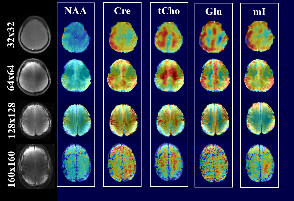
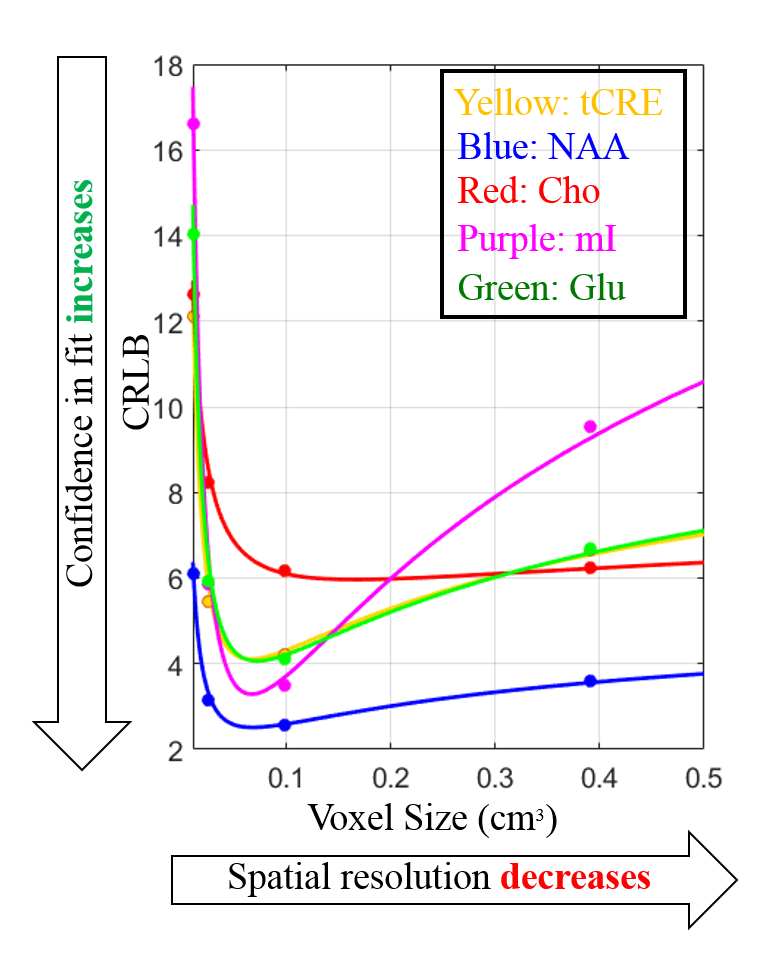
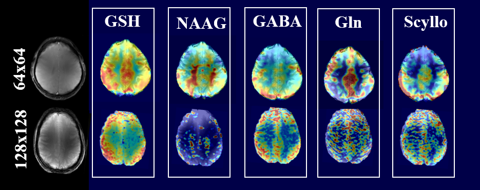
Figure 1 shows the metabolite maps of 5 major metabolites acquired at 9.4T for 4 increasingly higher spatial resolutions. Up to the resolution of 128x128, the maps show good anatomical correspondence, and the higher resolution maps reveal more anatomical details. Gray and white matter contrast for metabolites like Cre, Glu and Cho are observed both in accelerated (Figure 4) and non-accelerated (Figure 1) versions of these maps. However, at the resolution of 160x160, the drop in SNR due to the smaller voxel size dominates and the quality of the maps start deteriorating. From the clear trade-off between the higher spatial resolution and the SNR, one can quantitatively deduce the optimal resolution for metabolite mapping at 9.4T. Figure 2 shows plots of CRLB vs. voxel-size for 5 major metabolites. One can conclude that the optimal spatial resolution that would give us the most anatomical details while keeping the CRLB low is between the 64x64 and 128x128 spatial resolution. Figure 3 shows a maps of 5 lower concentrated metabolites acquired at these two resolutions at 9.4T. It can be seen that there is again a trade-off between SNR and high spatial resolution for mapping these metabolites.

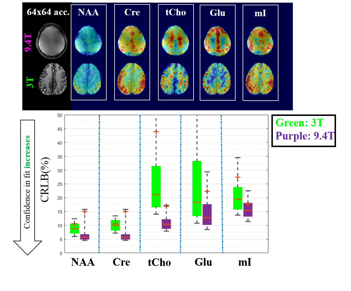
Next, to compare the quality of the maps at 9.4T to those acquired at the highest spatial resolution possible at 3T, Figure 4 shows a comparison between the maps acquired at a resolution of 64x64 on both scanner. The box plot shows the CRLB values across the slice for each metabolite on both scanners. It can be seen that even though visually the maps look comparable, the 9.4T fits have lower CRLBs and hence are more reliable.

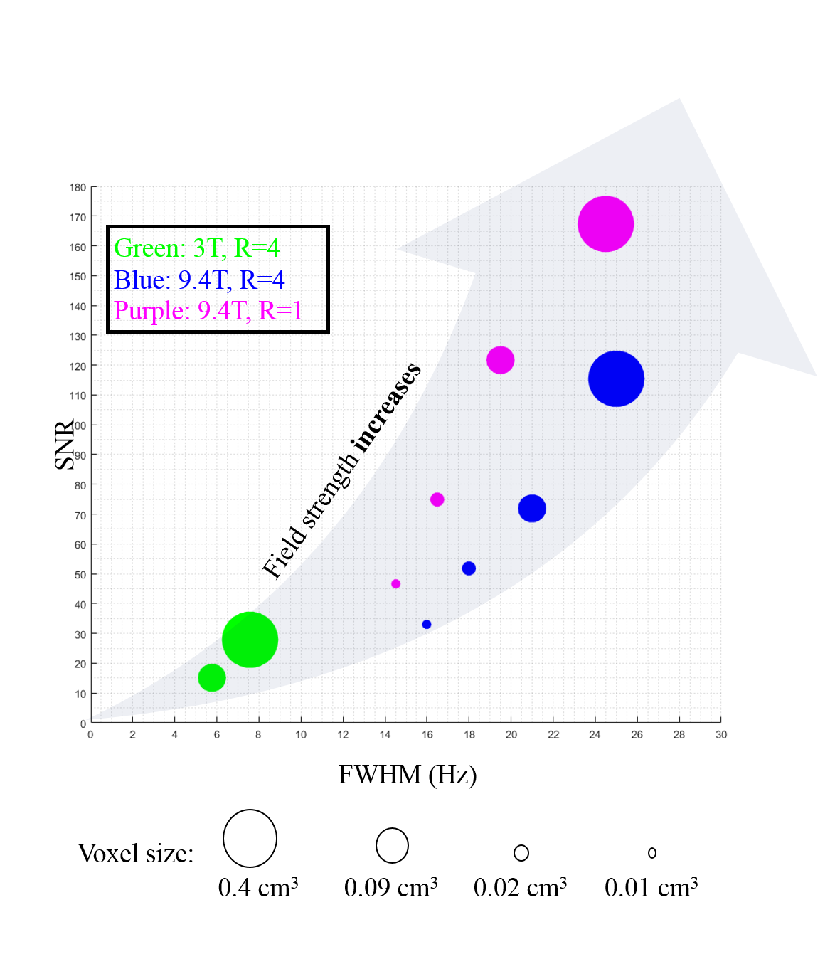
Finally, Figure 5 summarizes the results by plotting the SNR versus FWHM. The size of the dots correspond to the voxel-size. A clear trend in SNR gain and FWHM increase is seen as the field strength increases and an opposite trend is seen as we go to higher spatial resolutions.

Conclusion

Acknowledgements

References

[1] Henning et al, NMR Biomed 2009 [2] Bogner et al, MRM 2012 [3] Boer et al, MRM 2012 [4] Shajan et al, MRM 2014. [5] Hangel et al, NMR in Biomed 2015 [6] Bydder et al., MRI 2008 [7] Cabanes et al, JMR 2001 [8] Kay, Prentice Hall 1998