1233

A Hyperpolarized ¹³C MRI Approach for Calculating Glomerular Filtration Rate

Eugene Milshteyn^1,2, Cornelius von Morze¹, Jeremy W. Gordon¹, Galen D. Reed³, Robert A. Bok¹, and Daniel B. Vigneron^1,2

¹Radiology and Biomedical Imaging, UCSF, San Francisco, CA, United States, ²UC Berkeley-UCSF Graduate Program in Bioengineering, UCSF and University of California, Berkeley, San Francisco, CA, United States, ³HeartVista Inc., Los Altos, CA, United States

Synopsis

The feasibility of calculating glomerular filtration rate (GFR) using hyperpolarized ¹³C MRI is demonstrated in this project. HP001 is exhibited as a potential probe for GFR calculation due to its long T₁, allowing for high spatiotemporal resolution, and favorable filtration properties. Multiple iterations of common clinical sequences, including EPI and bSSFP, were utilized, and each sequence yielded GFR values close to those found in literature. The results shown here indicate potential for a new noninvasive imaging measurement of GFR.

Purpose

Glomerular filtration rate (GFR) is an important diagnostic marker for assessing renal function.¹ Several non-MR methods have been described to calculate GFR, including creatinine clearance, inulin clearance, and renal scintigraphy.¹ However, these methods suffer from various drawbacks, including invasiveness due to repeated urine and blood sampling, only providing global assessments of GFR, and exposing patients to ionizing radiation and potential nephrotoxicity.^1–3 Recently, gadolinium-based dynamic contrast enhanced MRI has provided a noninvasive method for calculating single-kidney GFR with adequate spatial resolution, but also has inherent drawbacks, including lowered SNR with increased renal impairment, long scan times, complex data analysis, and potential risk of nephrogenic systemic fibrosis in patients with low GFR.^2,4,5 New developments in hyperpolarized (HP) ¹³C molecular imaging has enabled real-time monitoring of various physiological processes within the context of disease progression.⁶ HP001 ( [¹³C]HMCP; hydroxymethyl cyclopropane; or bis-1,1-(hydroxymethyl)-[1-¹³C]cyclopropane-d₈) is a well-studied exogenous perfusion agent that is neither reabsorbed nor secreted by the kidney and appears to be freely filtered by the glomeruli, making it an excellent candidate for GFR measurements with HP MRI.⁷ In this study, we investigated the feasibility of using HP ¹³C MRI with HP001 to measure GFR in healthy Sprague-Dawley rats.

Methods

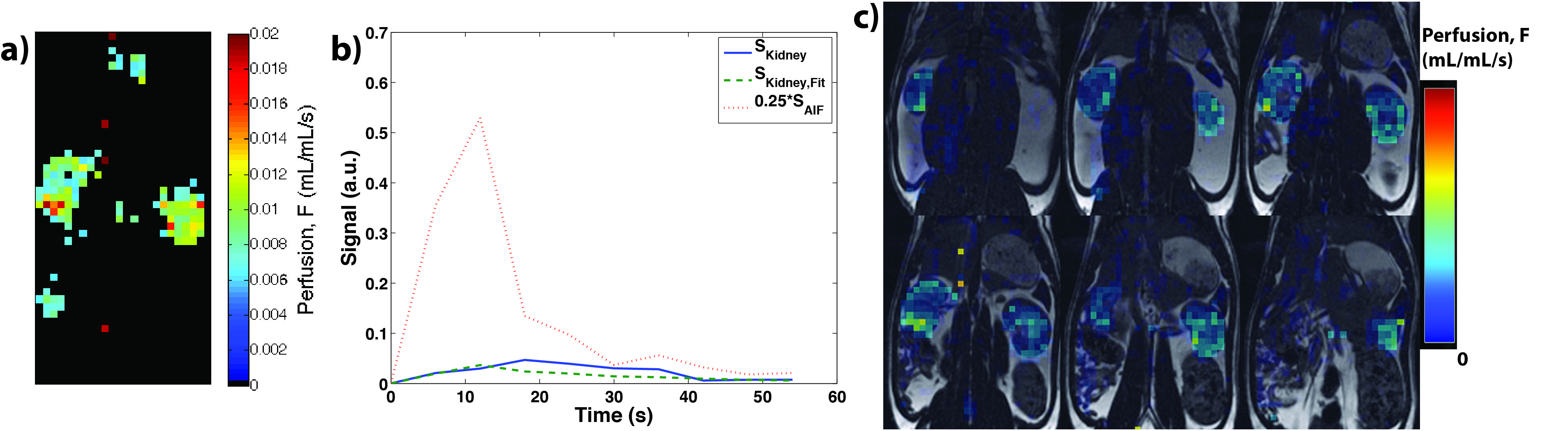
To calculate the kidney perfusion, F (mL/mL/s), the HP001 data was modeled with a simplified single-compartment model⁸ represented by the following differential equation:

$$\frac{dC_{tissue}(t)}{dt} = FC_{plasma}(t) - R_{1}C_{tissue}(t)$$

where C_tissue is the HP001 concentration in kidney (MR signal/mL), C_plasma is the arterial input function (AIF) (MR signal/mL), and R₁ is equal to 1/T_1,HP001. The solution to the differential equation,

$$C_{tissue}(t) = (1-v_{b})Fexp(-tR_{1})\otimes C_{plasma}(t)+v_{b}C_{plasma}(t)$$

which includes a blood volume v_b term (mL/mL), was used to fit HP001 dynamic curves via nonlinear least squares in Matlab. F_mean was calculated as the mean perfusion in the renal cortex and converted to GFR in mL/min/100g body weight by multiplying by 60s/min and the renal cortex volume in mL, and dividing by rat body weight.^9,10

Prospective acquisitions utilized either a slice-selective 2D balanced steady-state free precession (bSSFP) or symmetric, ramp-sampled echo planar imaging (EPI) sequence¹¹, or a 3D bSSFP sequence. The 2D acquisitions had the following parameters: 6.4x6.4 cm², 32x32 matrix size, 35mm axial slice covering both kidneys, progressive flip angle scheme,¹² 1-3s temporal resolution, 20-60 timepoints. In one animal, a variable temporal resolution scheme (0-4-8-9-10-11-12-13-14-15-16-17-18-24-30-36-…-60s) was utilized to better define the AIF. The 3D bSSFP had the following parameters: 12x6x2 cm³, 48x24x8 matrix size, 4-fold undersampling, progressive flip angle scheme,¹³ 6s temporal resolution, 10 timepoints. A maximum intensity projection image was used to calculate the mean perfusion from the 3D bSSFP data. ¹H 3D axial time-of-flight MR angiography images were also acquired to help define the AIF vessel size. The experiments were conducted on a 3T MR scanner and DNP experiments used a HyperSense polarizer. The scans started at the beginning of injection and 3mL of 100mM HP001 was injected over 12s via tail vein catheters in four different Sprague-Dawley rats (average body weight: 515g). The rats were kept under 1.5-1.75% isoflurane and 1mL/min of O₂ for the duration of the experiments.

Results and Discussion

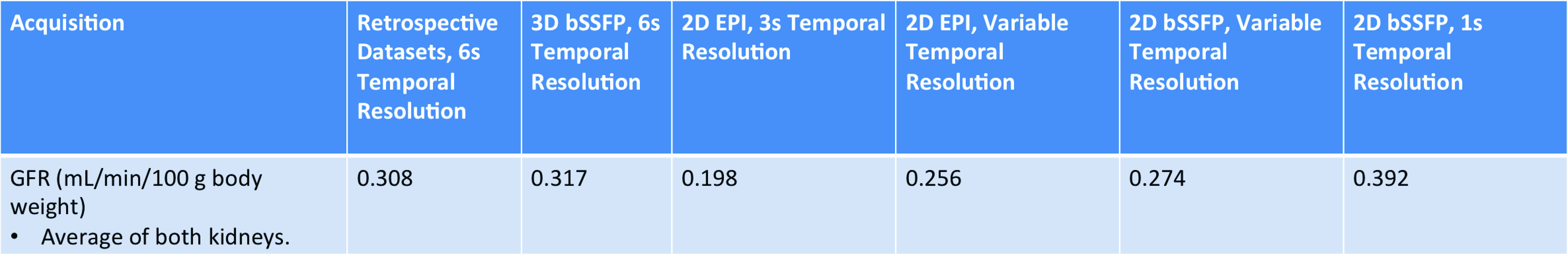
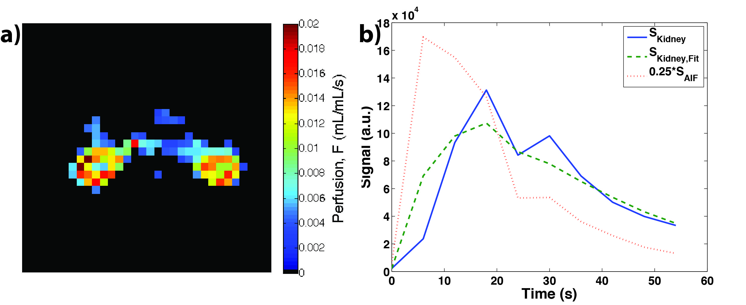
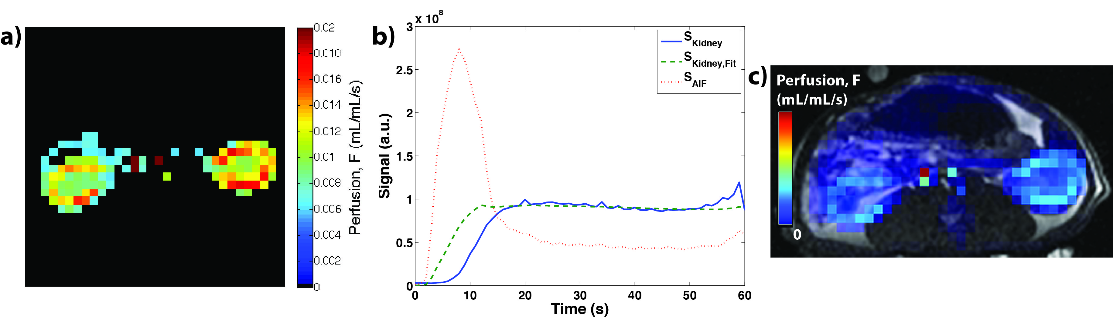
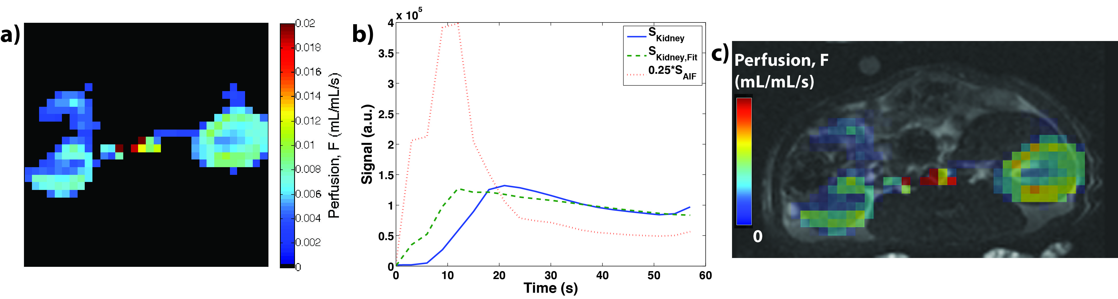
Table 1 summarizes the calculated GFR from both retrospective¹³ (four previously acquired HP001 datasets) and prospective acquisitions, which are similar to those found in literature (range of about 0.35-1.2+ mL/min/100g body weight for rats, depending on methodology).^10,14–16 Figures 1-4 depict the kidney perfusion, representative dynamic signal curves and associated fits, and perfusion overlays on ¹H images for a retrospective dataset, 2D bSSFP (1s temporal resolution), 2D EPI (variable temporal resolution), and 3D bSSFP acquisitions, respectively.

The methods presented here showed a wide range of calculated GFRs (0.198-0.392 mL/min/100g), which can be attributed to various factors that need to be further investigated: definition of AIF, spatiotemporal resolution, amount of temporal samples, SNR of the acquisition, use of single-compartment modeling, and any differences in renal function among the studied rats. Thus, future studies will also compare the calculated GFR from HP ¹³C MRI to a non-MR accepted standard, such as creatinine or inulin clearance. Furthermore, our study used isoflurane for anesthesia, which has been shown to reduce GFR by ~10%, ¹⁷ meaning the results presented here might slightly underestimate the true GFR. Future studies will investigate possible non-inhalant anesthesia, such as ketamine, for GFR calculation in rats.

Conclusion

In this study, we demonstrated feasibility to calculate GFR using HP ¹³C methods, indicating potential for a new noninvasive imaging tool for monitoring renal function. HP001 is a good candidate for GFR measurement, owing both to its filtration characteristics and its long T₁, which allows for high spatiotemporal imaging.

Acknowledgements

The authors would like to thank Mark Van Criekinge, Lucas Carvajal, and Zihan Zhu for all their help and funding from the NIH (P41EB013598 and R01EB017449).

References

1. Stevens, L. A. & Levey, A. S. Measured GFR as a Confirmatory Test for Estimated GFR. J. Am. Soc. Nephrol. 20, 2305–2313 (2011).

2. Bokacheva, L., Rusinek, H., Zhang, J. L. & Lee, V. S. Assessment of Renal Function with Dynamic Contrast Enhanced MR Imaging. Magn. Reson. Imaging Clin. N. Am. 16, 1–26 (2009).

3. He, X., Aghayev, A., Gumus, S. & Bae, K. T. Estimation of Single-Kidney Glomerular Filtration Rate without Exogenous Contrast Agent. Magn. Reson. Med. 71, 257–266 (2014).

4. Zhang, J. L. et al. Functional Assessment of the Kidney From Magnetic Resonance and Computed Tomography Renography: Impulse Retention Approach to a Multicompartment Model. 288, 278–288 (2008).

5. Kiani, S., Gordon, I., Mendichovszky, I., Cutajar, M. & Wells, K. Variation in GFR estimates derived from DCE-MRI renography studies in the presence of reduced Signal to Noise Ratio. in Proceedings of the International Society for Magnetic Resonance in Medicine 19 (2011) 814.

6. Kurhanewicz, J. et al. Analysis of cancer metabolism by imaging hyperpolarized nuclei: prospects for translation to clinical research. Neoplasia 13, 81–97 (2011).

7. Von Morze, C. et al. Simultaneous Multiagent Hyperpolarized ¹³C Perfusion Imaging. Magn. Reson. Med. 72, 1599–1606 (2014).

8. De Langen, A. J., Van Den Boogaart, V. E. M., Marcus, J. T. & Lubberink, M. Use of H₂¹⁵O-PET and DCE-MRI to Measure Tumor Blood Flow. Oncologist 13, 631–644 (2008).

9. Annet, L., Hermoye, L. & Peeters, F. Glomerular Filtration Rate: Assessment With Dynamic Contrast-Enhanced MRI and a Cortical-Compartment Model in the Rabbit Kidney. J. Magn. Reson. Imaging 20, 843–849 (2004).

10. Zöllner, F. G. et al. Functional imaging of acute kidney injury at 3 Tesla: Investigating multiple parameters using DCE-MRI and a two-compartment filtration model. Zeitschrift fßr Medizinische Phys. 25, 58–65 (2015).

11. Gordon, J. W., Vigneron, D. B. & Larson, P. E. Z. Development of a Symmetric Echo Planar Imaging Framework for Clinical Translation of Rapid Dynamic Hyperpolarized ¹³C Imaging. Magn. Reson. Med. 1–7 (2016). doi:10.1002/mrm.26123

12. Xing, Y., Reed, G. D., Pauly, J. M., Kerr, A. B. & Larson, P. E. Z. Optimal variable flip angle schemes for dynamic acquisition of exchanging hyperpolarized substrates. J. Magn. Reson. 234, 75–81 (2013).

13. Von Morze, C. et al. Investigating tumor perfusion and metabolism using multiple hyperpolarized ¹³C compounds: HP001, pyruvate and urea. Magn. Reson. Imaging 30, 305–311 (2012).

14. Sadick, M. et al. Original Articles Two non-invasive GFR-estimation methods in rat models of polycystic kidney disease: 3.0 Tesla dynamic contrast-enhanced MRI and optical imaging. Nephrol. Dial. Transplant. 26, 3101–3108 (2011).

15. Carrara, F. & Nattino, G. Simplified Method to Measure Glomerular Filtration Rate by Iohexol Plasma Clearance in Conscious Rats. Nephron 133, 62–70 (2016).

16. Solomon, S. Developmental Changes in Nephron Number, Proximal Tubular Length and Superficial Nephron Glomerular Filtration Rate of Rats. J. Physiol. 272, 573–589 (1977).

17. Grimm, K., Tranquilli, W. & Lamont, L. Essentials of Small Animal Anesthesia and Analgesia. (2011).

Figures

Table 1: Summary of GFR calculations (average of both kidneys) from both retrospective and prospective acquisitions. All prospectively acquired data, as well as retrospective data, provided GFR values that were close to the range found in literature for Sprague-Dawley rats. The highest value was calculated with the 2D bSSFP, 1s temporal resolution sequence, potentially due to having the smallest temporal resolution and largest amount of temporal samples. However, differences in these values can also be attributed to different timings, spatial resolution, and the rat studied, indicating a future need to compare these HP ¹³C measurements to non-MR GFR measurements.

Figure 1: Representative perfusion map acquired from a retrospective HP001 dataset. Part a depicts the perfusion in both kidneys, with relatively higher perfusion visible in the renal cortex. Part b depicts a representative dynamic HP001 signal curve (blue) and resulting fit (green) from one kidney, along with the arterial signal curves in red. The fit appears to match up closely with the acquired data, even with only 10 temporal samples and 6s temporal resolution.

Figure 2: The results from the prospective 2D bSSFP, 1s temporal resolution are shown here. a) perfusion in both kidneys, with relatively higher perfusion again visible in the renal cortex. b) Representative dynamic HP001 signal curve (blue) and resulting fit (green) from one kidney, along with the arterial signal curves in red. The fit here appears to match up closely with the acquired data. c) Overlay of part a on an axial ¹H image, with the ¹³C renal cortex pixels clearly overlaying on the ¹H renal cortex.

Figure 3: The results from the prospective 2D EPI, variable temporal resolution dataset are shown here. Parts a-c are similar as in Figure 2. A spline interpolation was done to recreate the data having constant 3s temporal resolution for fitting purposes. The variable temporal resolution allowed better definition of the arterial input function for better fitting, and could be a useful approach for optimal use of hyperpolarized magnetization to increase the temporal imaging window without sacrificing the fine temporal sampling needed for AIF definition.

Figure 4: The results from the prospective 3D bSSFP, 6s temporal resolution dataset are shown here. a) Maximum intensity projection of the coronal slices of the 3D acquisition. b) Representative dynamic HP001 signal curves from one kidney slice. c) ¹³C perfusion overlays on ¹H images, with multiple slices of the 3D acquisition shown. While the acquisition had lower SNR due to higher 3D spatial resolution, the calculated GFR values were similar to other sequences. This indicates potential for a 3D HP ¹³C MRI approach to calculating GFR and monitoring renal function.

Proc. Intl. Soc. Mag. Reson. Med. 25 (2017)

1233