Synopsis

One of the challenges MRF faces is the amount of data needed to be stored, loaded, and processed, especially when a high resolution dictionary is needed or large multi-dimensional analyses need to be taken into account. A low rank approximation to the high resolution MRF dictionary using a coarse dictionary is an effective remedy to this problem. Here we present one of many possible ways to implement low rank approximation to an arbitrary fine MRF dictionary by a coarse dictionary equipped with polynomial fitting, so as to avoid the need of pre-calculating, storing, and processing the large, finely-resolved MRF dictionary.

Purpose

Magnetic Resonance Fingerprinting (MRF) ¹ is a new quantitative MRI technique that matches the signal evolution for each voxel against a pre-calculated dictionary based on Bloch equation simulations with different combinations of parameters of interest, such as $T_1$, $T_2$, and off-resonance. One of the challenges it faces is the amount of data needed to be stored, loaded, and processed, especially when a high resolution dictionary is needed or large multi-dimensional analyses need to be taken into account ².

A low rank approximation to the high resolution MRF dictionary using a coarse dictionary is an effective remedy to this problem. Here we present one of many possible ways to implement low rank approximation to an arbitrary fine MRF dictionary by a coarse dictionary equipped with polynomial fitting, so as to avoid the need of pre-calculating, storing, and processing the large, finely-resolved MRF dictionary.

Methods

Consider an MRF-FISP ³ dictionary $D\in\mathbb{C}^{t\times n}$ with $T_1$ varying from 20ms to 1,940ms with a step size of 80ms and $T_2$ varying from 10ms to 170ms with a step size of 40ms ($T_2\le T_1$), where $t=3,000$ is the number of time frames and $n=119$ is the number of tissue type parameters. Let $D\approx U\Sigma V^*$ be the rank 3 randomized SVD ⁴ approximation of $D$, where $\cdot^*$ denotes the adjoint operator. We project the row space of $D$ into a 3-dimensional space by $X=U^*D$. We then fit the projected data with a degree 5 polynomial, resulting in a 4 times finer approximate dictionary (for a fair comparison against a 4 times finer dictionary of size $3,000\times1,585$ with step sizes of 20ms and 10ms for $T_1$ and $T_2$ respectively).

Now for a projected voxel evolution signal $\boldsymbol{s}$, it is first matched against all $T_1$, $T_2$ grids using maximal correlation to obtain the largest two $T_1$ values and two $T_2$ values (corresponding to the coarse dictionary) respectively. We then partition the fitted $T_1$ curves between the two fitted $T_2$ curves into $p=4$ even segments and find on each $T_1$ curve the point with the largest correlation with $\boldsymbol{s}$. Record the indices of these two points as $i$ and $j$ ($i, j=1,\ldots,p+1$). Then the $T_2$ value corresponding to $\boldsymbol{s}$ is estimated as $(T_{2,2}-T_{2,1})\times(i+j-2)/(2p)+T_{2,1}$. The $T_1$ value corresponding to $\boldsymbol{s}$ is estimated similarly.

To validate our model, we match an in vivo brain dataset of a healthy volunteer against a coarse dictionary, a fitted dictionary, and a dictionary that is 4 times finer than the coarse dictionary. The dataset is obtained on a Siemens Skyra 3T scanner (Siemens Healthcare, Erlangen, Germany) using the MRF-FISP sequence with a matrix size of $256\times 256$ and a field-of-view of 30cm². The brain data is also projected into the 3-dimensional random SVD space before matched against different dictionaries.

Results

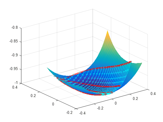
Fig.1 shows a 3D visualization of the projected randomized SVD space of the coarse MRF-FISP dictionary fitted with a degree 5 polynomial with fitting statistics $R^2=1$ and adjusted $R^2=0.99$. The cyan and red curves represent different $T_1$ and $T_2$ values respectively, and the circles represent fitted values along each curve, partitioning each coarse grid into 4 segments. The figure shows that the projected coarse dictionary fits the polynomial surface perfectly.

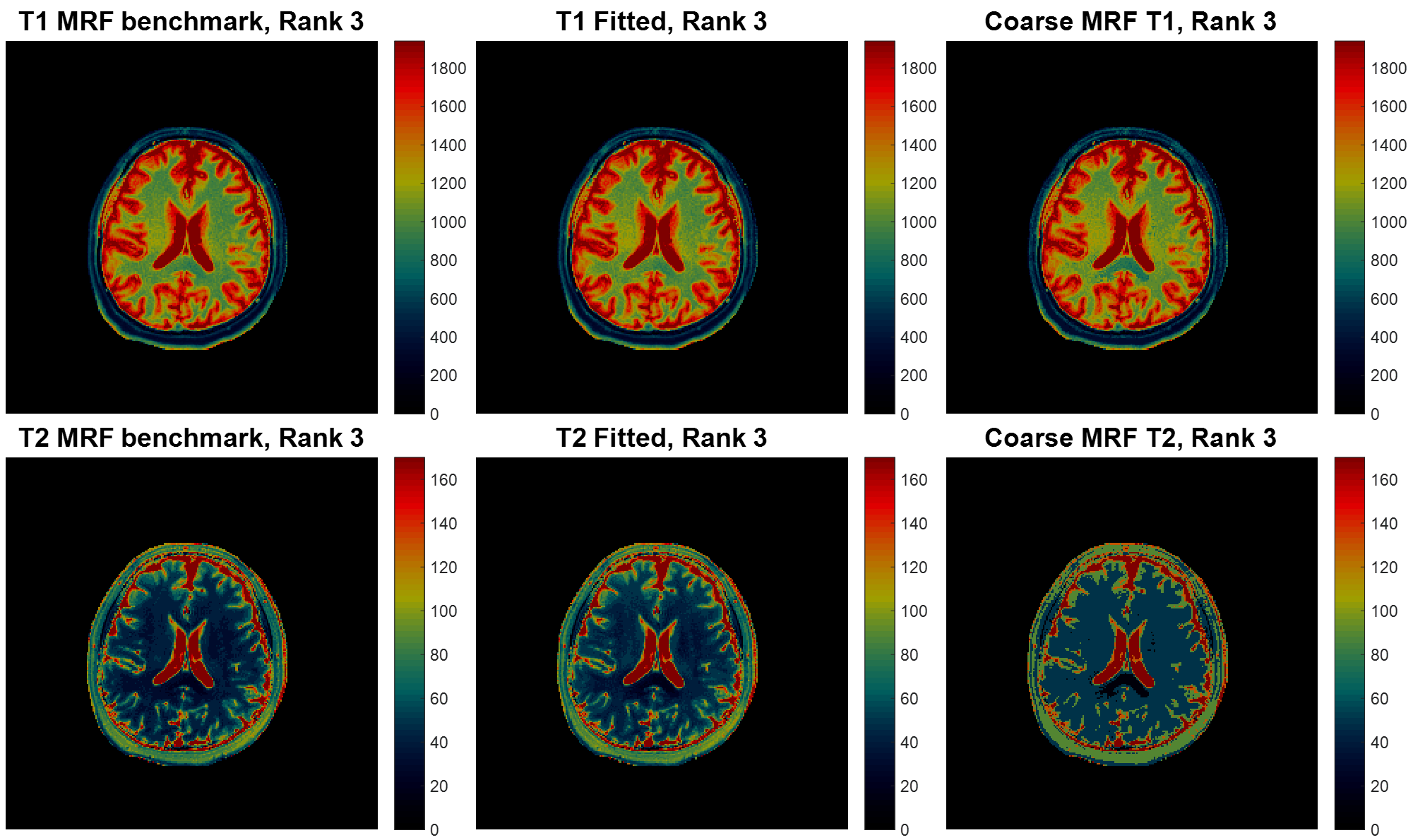
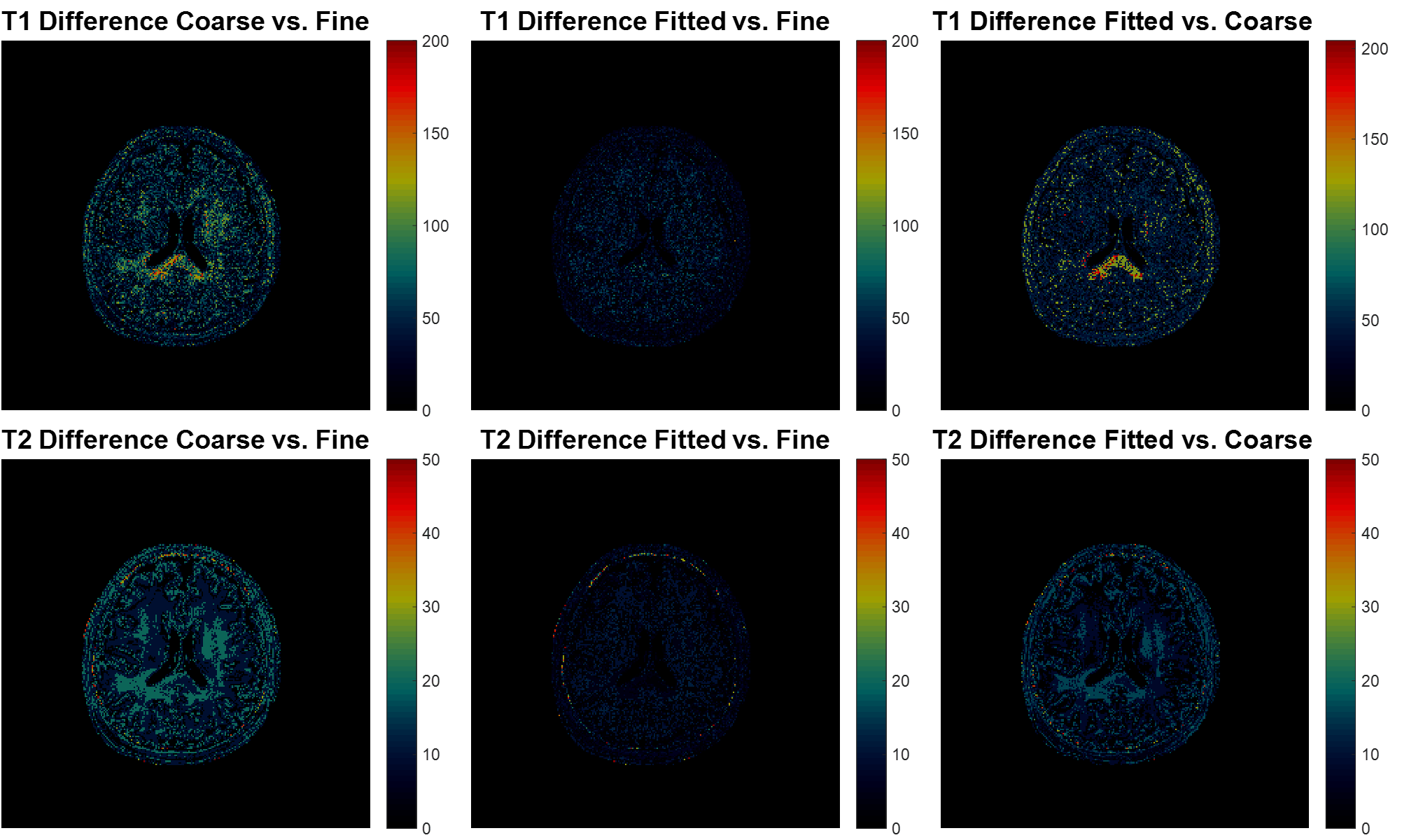
The MRF results with different dictionaries are shown in Fig.2 and Fig.3. In Fig.2, the $T_1$, $T_2$ maps of a scanned human brain are obtained via the projected coarse dictionary, the projected coarse dictionary fitted with a degree 5 polynomial, and the projected fine dictionary. We see a clear quality degradation when the dictionary is coarse. This, however, is remediated by fitting a polynomial to the coarse dictionary. The results are more clearly displayed in the difference maps in Fig.3. The $T_1$, $T_2$ map differences between the coarse dictionary and the 4 times finer dictionary are significantly diminished by the polynomial fitted dictionary.

Discussion and Conclusion

Acknowledgements

References

1. D. Ma, V. Gulani, N. Seiberlich, K. Liu, J. L. Sunshine, J. L. Duerk, and M. A. Griswold, Magnetic resonance fingerprinting. Nature 2013, 495:187–192.

2. J. Hamilton, A. Deshmane, M. A. Griswold, and N. Seiberlich, MR Fingerprinting with Chemical Exchange (MRF-X) for In Vivo Multi-Compartment Relaxation and Exchange Rate Mapping, Proc. Intl. Soc. Mag. Reson. Med. 24 (2016), 0431.

3. N. Halko, P. G. Martinsson, and J. A. Tropp, Finding Structure with Randomness: Probabilistic Algorithms for Constructing Approximate Matrix Decompositions, SIAM Review 2011 53:2, 217-288.

4. Y. Jiang, D. Ma, N. Seiberlich, V. Gulani, and M. A. Griswold, MR fingerprinting using fast imaging with steady state precession (FISP) with spiral readout. Magn. Reson. Med. 2015, 74: 1621–1631.