Synopsis

A new reconstruction method for accelerated J-resolved MRSI acquisitions is proposed. The proposed method performs a joint reconstruction from the data acquired with multiple echo times (TEs), using a formulation that integrates a subspace representation of the entire J-resolved spatiospectral function and a joint sparsity constraint exploiting the correlation across different TEs. Both simulation and in vivo experiments have been performed to evaluate the proposed method, demonstrating its superior performance over methods using joint sparsity or subspace constraint alone.

Introduction

Theory

The data acquired in a J-resolved MRSI experiment can be expressed as

\begin{eqnarray*}d(\mathbf{k},t_{2},t_{1}) & = & \int\rho\left(\mathbf{r},t_{2},t_{1}\right)e^{-i2\pi\Delta f(\mathbf{r})t_{2}}e^{-i2\pi\mathbf{k}\mathbf{r}}d\mathbf{r}+\varepsilon\left(\mathbf{k},t_{2},t_{1}\right)\quad\quad[1]\end{eqnarray*}

where $$$\rho(\mathbf{r},t_{2},t_{1})$$$ is the desired function, with $$$t_{2}$$$ the chemical shift time and $$$t_{1}$$$ the TE time (encoding J-coupling). $$$\Delta f(\mathbf{r})$$$ is the B₀ inhomogeneity and $$$\varepsilon(\mathbf{k},t_{2},t_{1})$$$ the measurement noise. Exploiting the spatiospectral correlations, the recently proposed SPICE method represents $$$\rho(\mathbf{r},t_{2})$$$ as $$$\rho(\mathbf{r},t_{2})=\sum_{l=1}^{L}u_{l}(\mathbf{r})v_{l}(t_{2})$$$ for a single $$$t_1$$$⁶. Here we extend this to model $$$\rho(\mathbf{r},t_{2},t_{1})$$$ as

\begin{eqnarray*}\rho\left(\mathbf{r},t_{2},t_{1}\right) & = & \sum_{l=1}^{L}u_{l}(\mathbf{r})v_{l}(t_{2},t_{1}).\quad\quad[2]\end{eqnarray*}

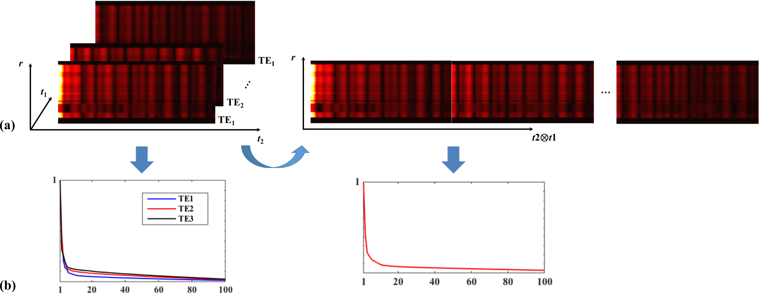
If $$$\boldsymbol{\rho}_{i}$$$ is a Casorati matrix representation of $$$\rho(\mathbf{r},t_{2},t_{1})$$$ at a particular $$$t_{1}$$$, the matrix representation of $$$\rho$$$ is a concatenation of $$$\boldsymbol{\rho}_{i}$$$'s, i.e., $$$\boldsymbol{\rho}=[\boldsymbol{\rho}_{1},\boldsymbol{\rho}_{2},\cdots,\boldsymbol{\rho}_{I_{1}}]$$$, with $$$I_{1}$$$ the total number of TEs (illustrated by Fig. 1). The above model can then be translated to $$$\boldsymbol{\rho}=\mathbf{U}\mathbf{V}$$$, where each row of $$$\mathbf{V}$$$ is a basis element in $$$\left\{ v_{l}(t_{2},t_{1})\right\}$$$.

Given this matrix representation, we formulate the reconstruction as follows

\begin{eqnarray*}\hat{\mathbf{U}} & = & \arg\underset{\mathbf{U}}{\min}\left\Vert \mathbf{d}-\mathcal{F}_{\Omega_{(k,t_{2},t_{1})}}\left\{ \mathbf{B}\odot\left(\mathbf{U}\mathbf{\hat{V}}\right)\right\} \right\Vert _{2}^{2}+\lambda\sum_{r=1}^{R}\left\Vert \mathbf{P}_{(r)}\right\Vert _{2}\\s.t. & & \mathbf{P}=\mathcal{\mathcal{R}}\left(\mathbf{D}\mathbf{U}\mathbf{\hat{V}}\right),\\\end{eqnarray*}

where $$$\hat{\mathbf{V}}$$$ is predetermined⁶, $$$\mathbf{B}$$$ a concatenation of $$$I_{1}$$$ matrices as $$$\left[\mathbf{B}_{0}\right]_{nm}=e^{-i2\pi\Delta f(\mathbf{r}_{n})t_{2,m}}$$$, and $$$\Omega_{(k,t_{2},t_{1})}$$$ a ($$$\mathbf{k}$$$,$$$t_{2}$$$,$$$t_{1}$$$)-space sampling operator. $$$\mathbf{D}$$$ computes finite differences and the regularization term is an $$$l_{2,1}$$$-norm penalty on $$$\mathbf{P}$$$, generated from $$$\mathbf{D}\mathbf{U}\mathbf{\hat{V}}$$$ by the operator $$$\mathcal{R}(.)$$$ which combines the folding of $$$\mathbf{D}\mathbf{U}\hat{\mathbf{V}}$$$ into a order-3 tensor and unfolding along the TE dimension. This is motivated by the assumption that images at different TEs should share similar edges, which has been previously used in parameter mapping and diffusion imaging^7,8. We solve this optimization problem using an alternating direction method of multipliers based algorithm.

Results

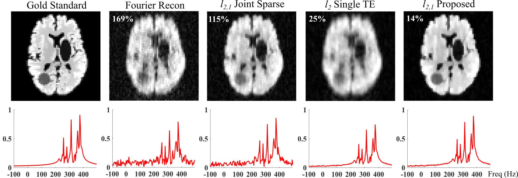
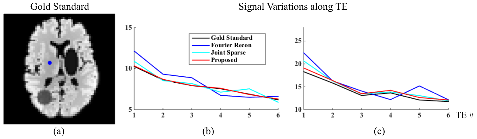
A numerical phantom was constructed to validate the proposed method. Spectra of several molecules for 6 different TEs were generated using GAVA⁹ and combined with different ratios. These synthesized spectra were assigned to different regions obtained by segmenting a brain image. Noise were added to simulate the measured ($$$\mathbf{k},t_{2},t_{1}$$$)-space data. A factor of three Gaussian undersampling was applied with different sampling patterns for each TE. Figures 2 and 3 compare the reconstructions obtained by different methods. As can be seen, a direct Fourier reconstruction yields very noisy and artifactual results. The proposed method offers the best performance (both quantitatively and qualitatively) compared to imposing joint sparsity or the subspace constraint alone.

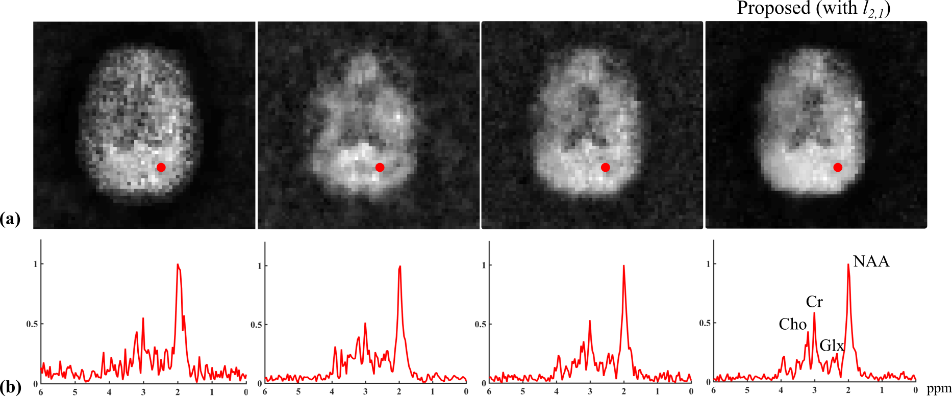
In vivo data were acquired from healthy volunteers on a Siemens 3T scanner (Trio). Accelerated high-resolution MRSI acquisition was done using a J-resolved spin-echo EPSI with the following parameters: 230x230mm² FOV, 10mm slice thickness, 64x64 matrix size, 120 echoes with 1.7ms spacing (x2 undersampling), 1200ms TR and 6 TEs (TE1=20ms, 30ms increment) with a 16min acquisition. The subspace for the proposed reconstruction was predetermined from training data acquired using a low-resolution EPSI scan with full spectral sampling (1500Hz bandwidth), matched TR/TEs, and 16x16 matrix size. Results were compared for a joint sparse reconstruction (very noisy), a TE-by-TE SPICE reconstruction⁶, a reconstruction using the model in Eq.[2] with $$$l_{2}$$$-regularization, and the proposed method (Fig. 4). Although no gold standard is available due to limited SNR, the proposed method produces reconstruction with the best SNR and spectral quality.

Conclusion

Acknowledgements

References

[1] de Graaf RA, In vivo NMR spectroscopy: Principles and techniques. Hoboken, NJ: John Wiley and Sons, 2007.

[2] Bolliger CS, Boesch C, and Kreis R, On the use of Cramér–Rao minimum variance bounds for the design of magnetic resonance spectroscopy experiments. NeuroImage, 2013;83:1031-1040.

[3] Li Y, Chen AP, Crane JC, Chang SM, Vigneron DB, and Nelson SJ, Three-dimensional J-resolved H-1 magnetic resonance spectroscopic imaging of volunteers and patients with brain tumors at 3T. Magn. Reson. Med., 2007;58:886-892.

[4] Wilson NE, Burns BL, Iqbal Z and Thomas MA, Correlated spectroscopic imaging of calf muscle in three spatial dimensions using group sparse reconstruction of undersampled single and multichannel data. Magn. Reson. Med., 2015;74:1199-1208.

[5] Ma C, Lam F, Liu Q, and Liang ZP, Accelerated high-resolution multidimensional 1H-MRSI using low-rank tensors. Proc. Intl. Soc. Mag. Reson. Med., 2016, p. 379.

[6] Lam F and Liang ZP, A subspace approach to high-resolution spectroscopic imaging. Magn. Reson. Med., 2014;71:1349-1357.

[7] Haldar JP, Wedeen VJ, Nezamzadeh M, Dai G, Weiner MW, Schuff N, and Liang ZP, Improved diffusion imaging through SNR-enhancing joint reconstruction. Magn. Reson. Med., 2013;69:277-289.

[8] Zhao B, Lu W, Hitchens TK, Lam F, Ho C, and Liang ZP, Accelerated MR parameter mapping with low-rank and sparsity constraints. Magn. Reson. Med., 2015;74:489-498.

[9] Soher BJ, Young K, Bernstein A, Aygula Z, and Maudsley AA, GAVA: spectral simulation for in vivo MRS applications. J. Magn. Reson., 2007;185:291-299.