1142
Three-dimensional Ultrashort Echo Time Cones Imaging with Magnetization Transfer Modeling (3D UTE-Cones-MT): Simulation, Specimen and Volunteer Studies of the Knee Joint1Radiology, University of California, San Diego, San Diego, CA, United States, 2Radiology Service, VA San Diego Healthcare System, San Diego, CA, United States, 3GE Healthcare, San Diego, CA, United States
Synopsis
A major limitation associated with conventional clinical MRI sequences is the magic angle effect . The conventional T2 and T1rho measures may increase more than 100% when the fibers are oriented from 0º to the magic angle (~55º) relative to the B0 field, far more than that associated with osteoarthritis (OA). Magnetization transfer (MT) imaging has shown less sensitivity to the magic angle effect, and can indirectly evaluate macromolecules which have extremely short T2 (~10 us) and invisible with all MRI sequences. However, conventional MT techniques cannot be applied to short T2 tissues such as menisci, ligaments, tendons and bone. Ultrashort echo time (UTE) sequences with TEs 100-1000 times shorter than those of clinical sequences have been developed to image these short T2 tissues. In this study, we aimed to develop 3D UTE with Cones sampling and MT (3D UTE-Cones-MT) imaging and signal modeling to quantify water and macromolecules in both short and long T2 tissues in the knee joint at 3T.
Introduction
A major limitation associated with conventional clinical MRI sequences is the magic angle effect (1). The conventional T2 and T1rho measures may increase more than 100% when the fibers are oriented from 0º to the magic angle (~55º) relative to the B0 field (2-4), far more than that associated with osteoarthritis (OA) (5). Magnetization transfer (MT) imaging has shown less sensitivity to the magic angle effect (6,7), and can indirectly evaluate macromolecules which have extremely short T2 (~10 us) and invisible with all MRI sequences (8). However, conventional MT techniques cannot be applied to short T2 tissues such as menisci, ligaments, tendons and bone. Ultrashort echo time (UTE) sequences with TEs 100-1000 times shorter than those of clinical sequences have been developed to image these short T2 tissues (9,10). In this study, we aimed to develop 3D UTE with Cones sampling and MT (3D UTE-Cones-MT) imaging and signal modeling to quantify water and macromolecules in both short and long T2 tissues in the knee joint at 3T.Methods and Materials
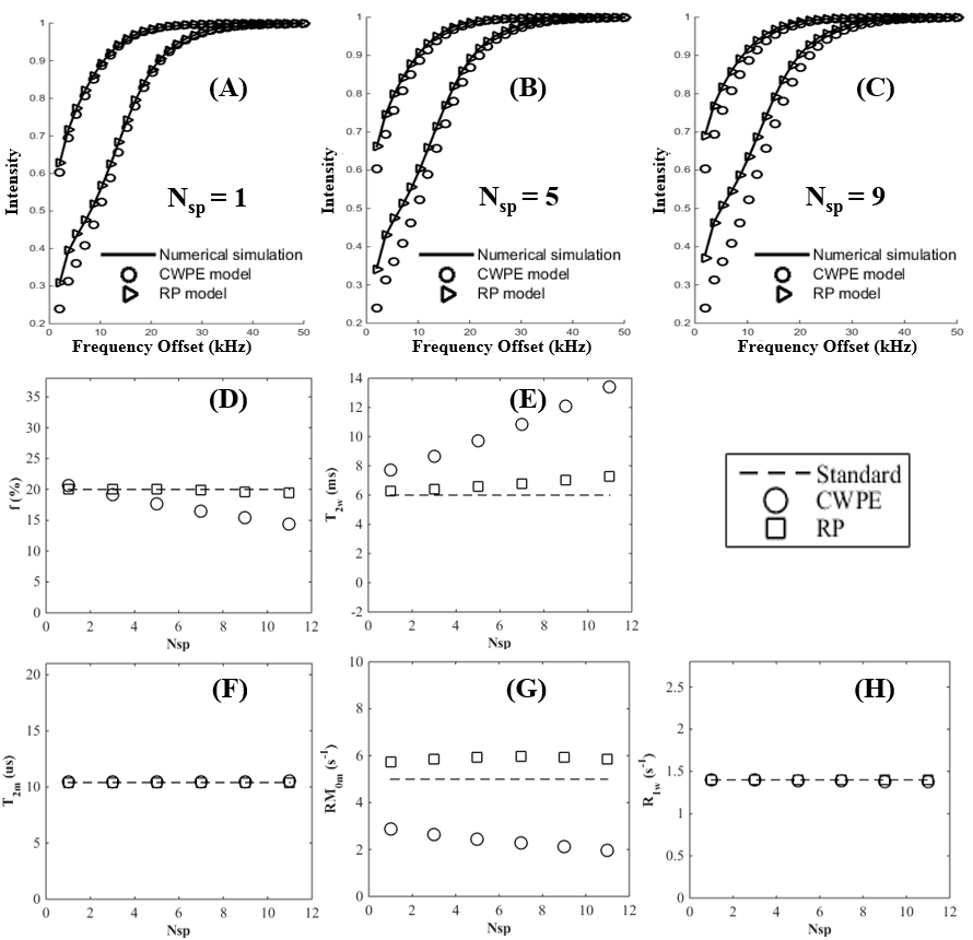
The 3D UTE-Cones-MT sequence employs a short pulse excitation followed by spiral trajectories with conical view ordering (11). The Cones images acquired with a series of MT pulse power (w1) and off-resonance frequencies (Df) were used for two-pool MT modeling to evaluate macromolecular proton fraction f and T2m, exchange rate RM0m and water longitudinal relaxation rate R1w. To reduce total scan time several spiral spokes (Nsp) were acquired after each MT preparation, thus scan time being reduced by a factor of Nsp. The effect of an MT pulse on the macromolecular pool is modeled as a rectangular pulse (RP approximation) whose width is equal to the full width at half maximum of the curve obtained by squaring the MT pulse throughout its duration. The RP pulse has equivalent average power to that of the original MT pulse, similar to the Sled and Pike model (12). Numerical simulation was performed to compare the new RP model with the continues wave power equivalent (CWPE) model (13). Both Gaussian and Super-Lorentzian lineshapes for the macromolecular pool were tested, followed by studying in vitro tendons, bone and knee joint samples (n=2), and finally the knee joint of healthy volunteers (n=5). Typical imaging parameters included: TR=100 ms, TE=32 µs, flip angle=7°, FOV=14 cm, slice thickness=2-3 mm, readout=256-320, slices=30-60; Nsp=9, two to three powers (500°-1500°) and five MT frequency offsets (2, 5, 10, 20 and 50 kHz), scan time of 5 (in vitro) to 2 min (in vivo) per acquisition. Mean and standard deviation of macromolecular proton fraction f, T2m, RM0m and R1w were calculated.Results
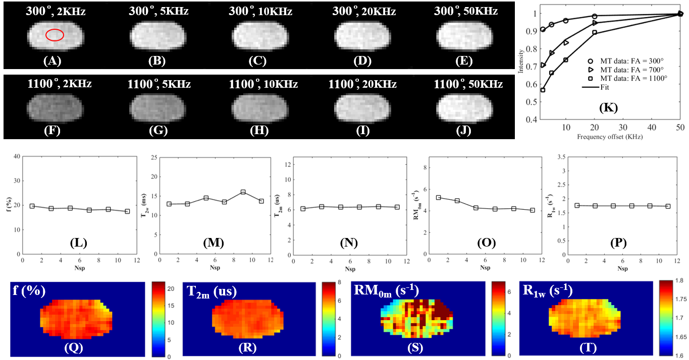
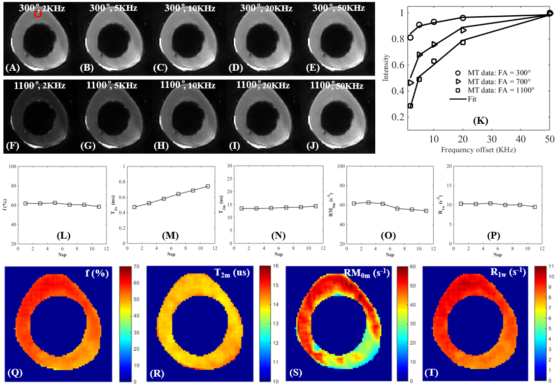
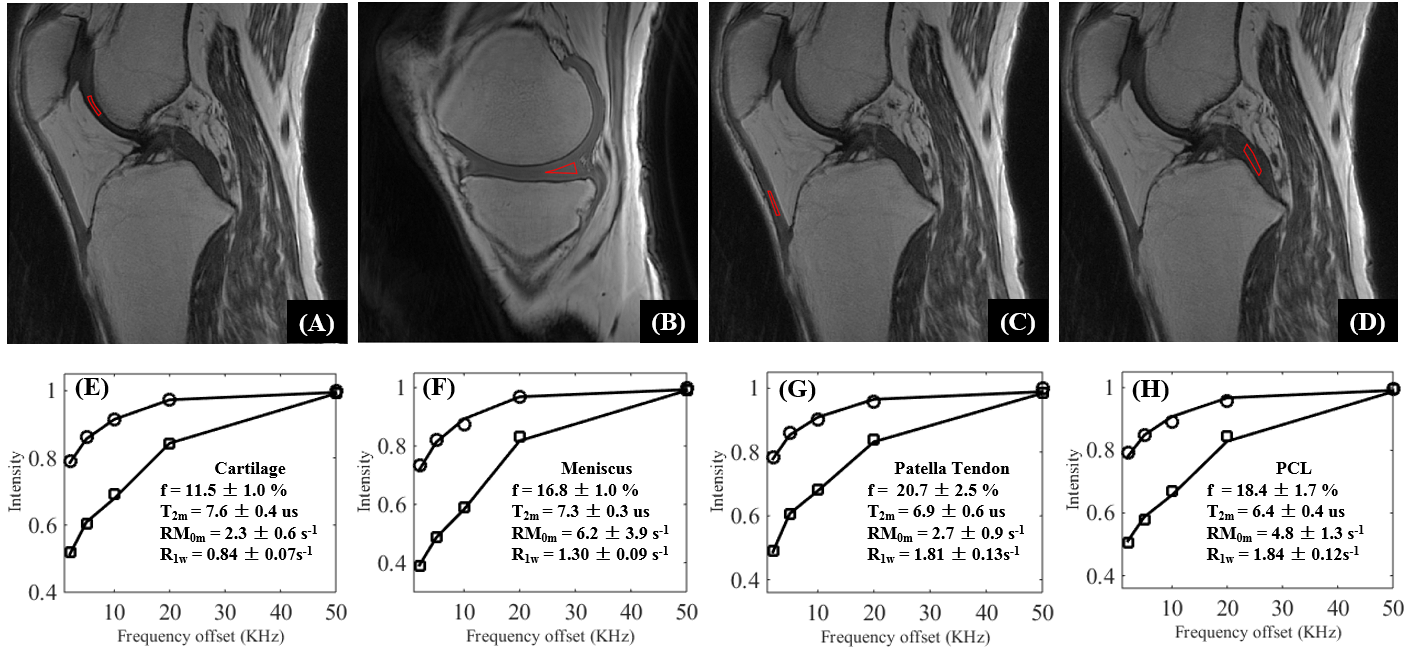
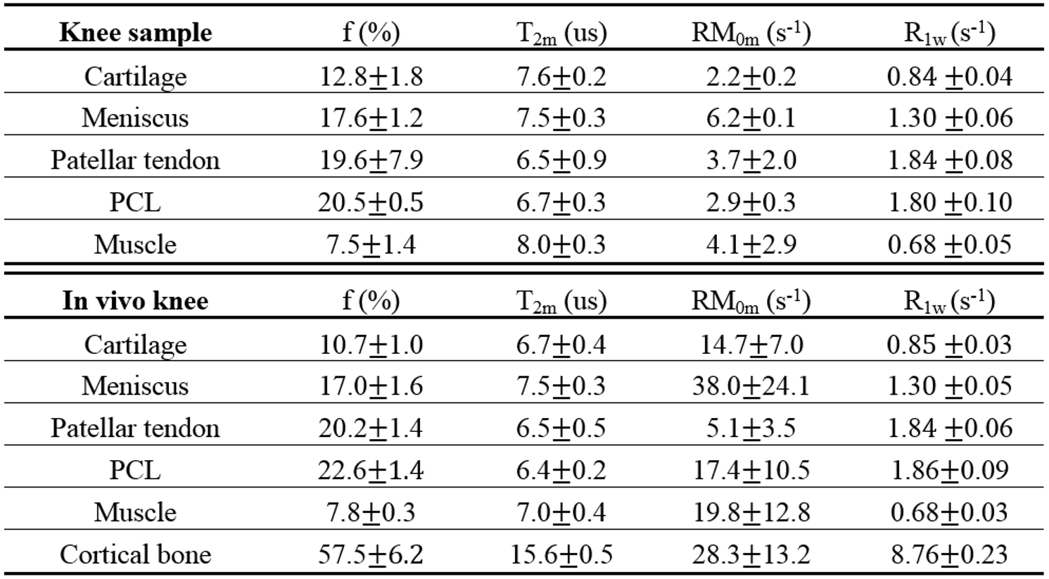
Simulation in Figure 1 shows that the RP model outperforms the CWPE model especially for higher Nsp. With a Nsp of 9, the CWPE model underestimates f by more than 25% and RM0m by 60%, and overestimates T2w by more than 50%. In comparison the RP model can accurately estimate all these parameters, with less than 3% error for f, T2m and R1w. Similar results were observed for the Gaussian lineshape. Figure 2 shows UTE-Cones-MT images of a tendon sample. A Super-Lorentzian lineshape was used for MT modeling. The MT parameters are relatively constant with different Nsp, consistent with simulation. Figure 3 shows UTE-Cones-MT images of a bovine bone sample. Cortical bone was depicted with high signal and resolution with all UTE-Cones-MT images. The collagen in cortical bone is more solid-like and a Gaussian lineshape was used for MT modeling. The lower half of this bovine cortical bone sample shows increased signal intensity, consistent with the reduced collagen proton fraction, RM0m and R1w. Figure 4 shows selected 3D UTE-Cones-MT images of the knee joint of a 45-year-old male donor. High-resolution volumetric images of the knee joint can be used for excellent two-pool MT modelling and curve fitting, providing quantitative evaluation of macromolecules and water components in major knee joint tissues. Table 1 summarizes the mean and standard deviation of two-pool MT modeling parameters in vitro and in vivo knee joints. The in vivo MT parameters are largely consistent with values from ex vivo studies, especially for f, T2m and R1w.Discussion and Conclusion
Simulation together with in vitro and in vivo studies demonstrate that the 3D UTE-Cones-MT imaging and two-pool modeling can be used for volumetric assessment of macromolecular and water components in both the short and long T2 tissues of the knee joint. And these biomarkers are magic angle insensitive. This technique is likely to help early detection of OA and monitoring the effects of therapy from a truly “whole-organ” approach.Acknowledgements
The authors acknowledge grant support from NIH (1R01 AR062581-01A1, 1 R01 AR068987-01) and VA Clinical Science R&D Service (Merit Award I01CX001388).References
1. Erickson SJ, Prost RW, Timins ME. The “magic angle” effect: background physics and clinical relevance. Radiology 1993; 188:23-25.
2. Xia Y, Farquhar T, Burton-Wurster N, Lust G. Origin of cartilage laminae in MRI. J Magn Reson Imaging 1997; 7:887-894.
3. Mlynarik V, Szomolanyi P, Toffanin R, Vittur F, Trattnig S. Transverse relaxation mechanisms in articular cartilage. J Magn Reson 2004; 300-307.
4. Du J, Statum S, Znamirowski R, Bydder GM, Chung CB. Ultrashort TE T1rho magic angle imaging. Magn Reson Med 2013;69(3):682-687.
5. Mosher TJ, Zhang Z, Reddy R, Boudhar S, Milestone BN, Morrison WB, Kwoh CK, Eckstein F, Witschey WR, Borthakur A. Knee articular cartilage damage in osteoarthritis: analysis of MR image biomarker reproducibility in ACRIN-PA 4001 multicenter trial. Radiology 2011; 258:832-842.
6. Li W, Hong L, Hu L, Maqin RL. Magnetization transfer imaging provides a quantitative measure of chondrogenic differentiation and tissue development. Tissue Eng Part C Methods 2010; 16:1407-1415.
7. Hopfgarten C, Kirsch S, Reisig G, Kreinest M, Schad LR. Identification of in vitro degenerated porcine meniscal tissue: MRT contrast prevents misinterpretation due to the magic angle effect. In: Proceedings of the 22nd Annual Meeting of ISMRM, Sydney, Australia, 2012, P1397.
8. Henkelman RM, Huang X, Xiang Q, Stanisz GJ, Swanson SD, Bronskill MJ. Quantitative interpretation of magnetization transfer. Magn Reson Med 1993;29:759–766.
9. Hodgson RJ, Evans R, Wright P, Grainger AJ, O'Connor PJ, Helliwell P, McGonagle D, Emery P, Robson MD. Quantitative magnetization transfer ultrashort echo time imaging of the Achilles tendon. Magn Reson Med 2011;65(5):1372-1376.
10. Ma Y, Shao H, Du J, Chang EY. Ultrashort Echo Time Magnetization Transfer (UTE-MT) Imaging and Modeling: Magic Angle Independent Biomarkers of Tissue Properties. NMR Biomed 2016; 29:1546-1552.
11. Carl M, Bydder GM, Du J. UTE imaging with simultaneous water and fat signal suppression using a time-efficient multispoke inversion recovery pulse sequence. Magn Reson Med 2016; 76:577-582.
12. Sled JG, Pike GB. Quantitative interpretation of magnetization transfer in spoiled gradient echo MRI sequences. J Magn Reson 2000;145:24–36.
13. Ramani A, Dalton C, Miller DH, Tofts PS, Barker GJ. Precise estimate of fundamental in-vivo mt parameters in human brain in clinically feasible times. Magn Reson Imag 2002;20:721–731.
Figures