1045
A scalable composite through-time radial GRAPPA method1Electrical and Computer Engineering, University of Minnesota, Minneapolis, MN, United States, 2Center for Magnetic Resonance Research, University of Minnesota
Synopsis
Through-time radial GRAPPA showed promising reconstruction for cardiac imaging. However, it's challenging to extend 3D Kooshball trajectory because of long calibration scans. We propose a novel and flexible data-driven calibration method. The MRXCAT numerical phantom image results show image similarity with through-time radial GRAPPA.
Introduction
The through-time radial GRAPPA [1] (TT-rGRAPPA) has shown success in dynamic cardiac imaging applications. However, the need for additional scans to acquire calibration frames makes it challenging to utilize when extra scans are not available, especially for dynamic 3D koosh-ball imaging. In this study, we propose a data-driven calibration method to calibrate region-specific GRAPPA kernels for radial acquisitions, with scalability to 3D koosh-ball trajectories.Methods
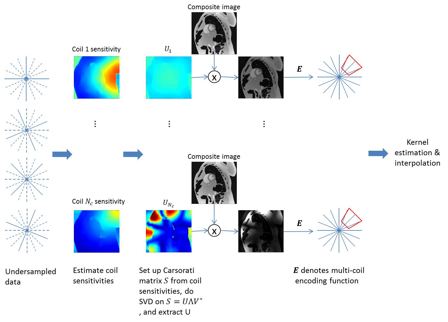
In TT-rGRAPPA method, there are two sequential phases: dynamic and calibration (Fig 1). The bit-reversed order is used in the dynamic phase to make incoherent motion artifacts. The linear order is used in the calibration phase without motion compensation since motion averages out in GRAPPA kernel estimation. In this phase, multiple fully-sampled radial datasets are acquired over time. The center black point denotes target point in missing locations. The surrounding black points refer to source points in acquired locations. After collection of sufficient calibration data, an over-determined linear system is formed and solved to obtain a region-specific GRAPPA kernel. Then these kernels are applied to corresponding location in undersampled data to reconstruct the missing points.
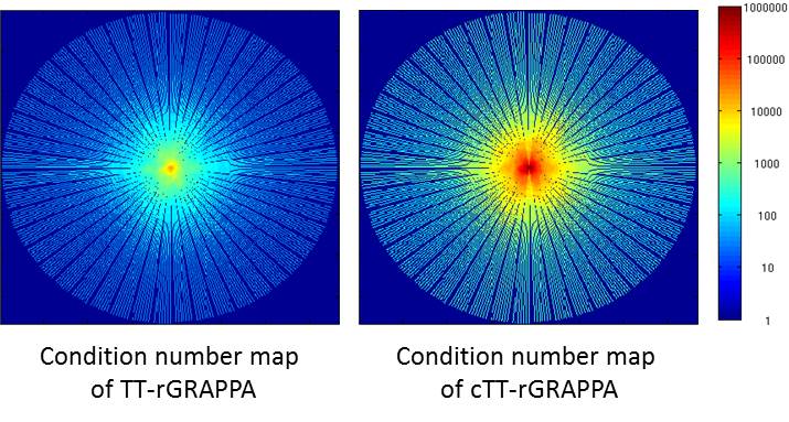
Because of the inherent time-averaging in through-time calibration, we propose to synthesize data-driven training datasets from the composite image. The proposed method (composite through-time radial GRAPPA, cTT-rGRAPPA) is described step by step in the flowchart (Figure 2). The number of the synthesized training datasets is equal to number of coils, . SVD is applied to generate unitary coil sensitivities matrices, which does not amplify noise in the composite image. To validate the proposed method, we used MRXCAT numerical phantom images [2]. The simulated data is generated by inverse gridding using the radial view ordering in Fig 1. The training data is synthesized through the proposed method. Then the region specific GRAPPA kernels are calibrated through an over-determined system. Unfortunately, the system has bad conditioning and the condition number map in k-space is shown in Fig 4. Hence, we use regularization to reduce dependencies between our synthetically generated calibration data. We also did experiment using 8 Biot-Savart coils under the same SNR as the abdomianl coil experiment and the RMSE result versus four different reduction factors is shown in Fig 5 bottom-right.
Results
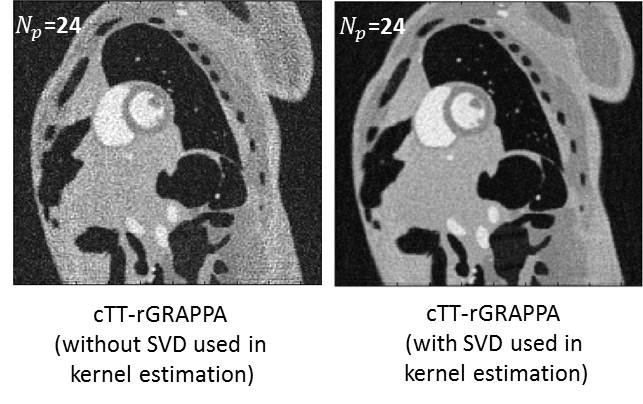
Fig. 3 shows image quality is improved when SVD is used to generate unitary coil sensitivity matrices to avoid noise amplification in the process of training data synthesis. The images are reconstructed from 24 projections (R=8) using cTT-rGRAPPA. Figure 5 shows the images reconstructed from undersampled data rate using three different radial GRAPPA methods under SNR=25. The coil sensitivity used to emulate physical coils are calibrated from a slice of 3D in-vivo dataset using 10 abdominal coils. The image size is 192x192. The sd-rGRAPPA denotes standard radial GRAPPA [4]. cTT-rGRAPPA has 1~2% higher RMSE than TT-rGRAPPA under four different reduction factors (R=8, 12, 16 and 24).
The use of abdominal coils, which are relative coils causes 1~2% higher RMSE than the Biot-Savart coil experiment for both TT-rGRAPPA and cTT-rGRAPPA methods. It is because relative coils have inhomogeneous B1 and Biot-Savart has homogeneous B1 .
Discussion
Proposed cTT-rGRAPPA enables calibration of GRAPPA kernels without requiring the acquisition of a long series of calibration data. Though it has an inherent limitation of bad conditioning due to correlated synthesized training datasets, this was mitigated using appropriate regularization. cTT-rGRAPPA enjoys the fast computation properties of rGRAPPA while providing scalability to 3D koosh-ball trajectories, since it does not require extra scans of multiple training data with the same trajectory.Acknowledgements
Center for Magnetic Resonance Research - BTRC (P41 EB015894)
References
1. Seiberlich et al., Improved radial GRAPPA calibration for real-time free-breathing cardiac imaging. MRM 2011
2. Wissman et al., MRXCAT: realistic numerical phantoms for cardiovascular magnetic resonance. J Cardiovasc Magn Reson 2014
3. Ding et al., Paradoxical effect of the signal-to-noise ratio of GRAPPA lines: a quantitative study. MRM 2014
4. Griswold et al, Direct parallel imaging reconstruction of radially sampled data using GRAPPA with relative shifts. Proc Intl Soc Magn Reson Med 2003
Figures