Synopsis

Magnetic resonance imaging based electrical conductivity imaging of biological tissues could be highly challenging at magnetic fields of the order of 18.8T. We could see significant magnetohydrodynamic (MHD) effects in low viscosity materials at such fields. In this study, we investigated these effects using saline and agarose phantoms and explained the MHD mechanism using a fluid flow model coupled with electromagnetic field equations. Experimental and simulation results showed a correlation between the higher magnetic field and velocity. This relation changed from exponential to linear as the viscosity of material increased. The velocity was negligible for highly viscous materials such as agarose.

Introduction

Methods

We developed two phantoms of 1 S/m conductivity with different viscosities, using either saline or agarose. We injected 200 $$$\mu$$$A current through carbon electrodes attached to phantom surface. A spin echo ICNE pulse sequence was used to acquire complex k-space data using a 18.8T vertical bore Varian MRI scanner². Our imaging parameters were: TR/TE=1000/20ms, imaging matrix=128×128, slice thickness=1mm, in-plane resolution=12×12mm2, number of averages=2. We collected data for two polarities of current injection with a total data acquisition time of 8min32s and calculated the z-component of the induced magnetic flux density (Bz)¹.

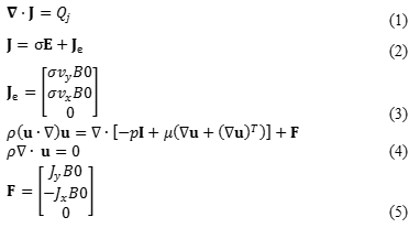
We developed a multi-physics model using a commercial software COMSOL (Comsol Inc, Burlington, MA, USA) by coupling the laminar flow equations with the electromagnetic field equations. The equations (1)-(5) in figure 4 explain the governing physics behind our MHD model. We assumed a domain $$$\chi$$$ having an electrical conductivity $$$\sigma$$$. We injected imaging current through surface electrodes, producing a current density J₁=$$$\sigma$$$E, an electric field E and electric potential u in $$$\chi$$$. The J₁ induced a magnetic flux density which interacted with the main magnetic field B0 of the MR scanner and produced a volume force F. This force created motion in the domain $$$\chi$$$ whose spatially varying velocity v_x,y depended on the viscosity in $$$\chi$$$. Depending on the strength of B0 and the amplitude of v_x,y , a secondary current density J_e was produced which created a secondary magnetic field.

In our model, we assumed the normal current density and ground to be the two electrical boundary conditions on two ports, and insulation elsewhere. An open boundary was specified at the top surface of $$$\chi$$$. The various boundary settings were: normal current density = 63.66 A/m², normal stress f₀ = 0 N/m², density of saline solution = 1000 kg/m³ and dynamic viscosity = 1 mPa s. By default, the laminar flow physics assumed a ‘Wall’ boundary condition in COMSOL. We specified ‘No Slip’ boundary conditions on all external boundaries, except at the open boundary of the saline or agar medium in $$$\chi$$$.

Results and Discussion

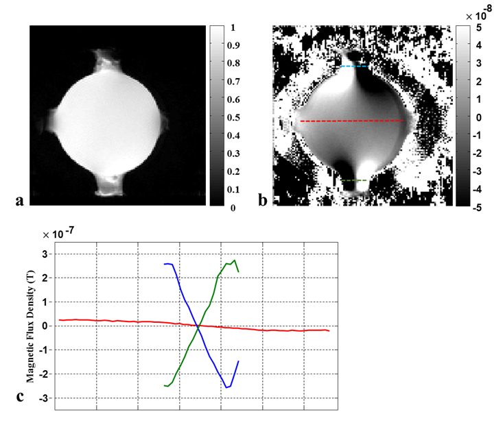
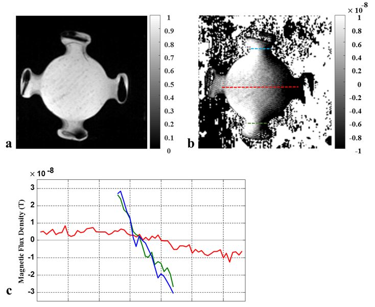
Figure 1 shows the experimental results of measuring the magnetic flux density from complex k-space MR images for saline phantom. The images in a, b are the MR magnitude and B_z respectively. The profiles in figure c compare the B_z at three different locations labelled in b. The images in figure 2 show the corresponding results for agarose phantom.

Comparing the B_z profiles in figure 1c and 2c, we note that the slopes of the saline phantom B_z distribution are opposite each other at the current injection and ground ports. This implies that there was no net current flow across the electrodes. Instead, the induced magnetic field circulated locally around each port. This phenomenon was not observed in agarose phantoms in figure 2.

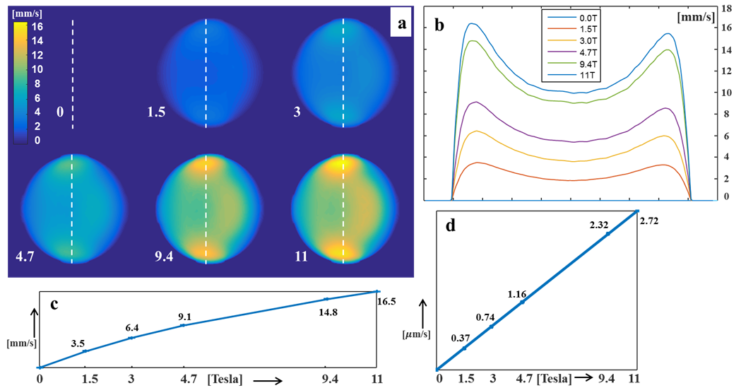
Figure 3 shows the MHD simulation results for the magnitude of velocity generated as a function of the external magnetic fields B0 = [0,1.5,3,4.7,9.4,11] Tesla for saline phantom (a-c). The maximum value of velocity (v_max) appeared closer to the ports of current injection and ground which indicates a strong motion around the ports. The v_max at 3T was 6.4 mm/s. We estimated the v_max to be 22.6 mm/s at 18.8T based on the exponential relation between B0 and velocity as can be seen in figure 3c. The exponential relation changed to linear relation in highly viscous materials like agarose with viscosity=10 Pa s (figure 3d). Using this relation, we estimated the v_max to be 4.7 $$$\mu$$$m/s at 18.8T.

Conclusion

Acknowledgements

References

1. Woo E J and Seo JK. Magnetic resonance electrical impedance tomography (MREIT) for high-resolution conductivity imaging. Physiol Meas. 2008;29(10):R1-26.

2. Minhas A S, Jeong W C, Kim Y T, et.al. Experimental performance evaluation of multi-echo ICNE pulse sequence in magnetic resonance electrical impedance tomography. Magn Reson Med. 2011;66(4):957-65.

3. Davidson P A. An Introduction to Magnetohydrodynamics. Cambridge University Press; 2001.