0994
Quantitative modeling of exchange in bSSFPX1Department of Radiology, UT Southwestern Medical Center, Dallas, TX, United States, 2Advanced Imaging Research Center, UT Southwestern Medical Center, Dallas, TX, United States
Synopsis
bSSFP was shown to be sensitive to exchange and is explored as an alternative way for CEST/T1ρ experiments (the bSSFPX method). In this abstract, an analytical solution is derived for the magnetization behavior in the bSSFPX. The solution describes the transient signal fluctuations for short saturation times. The solution is verified by comparing it to full, step-wise computation of Bloch-McConnell Equations. Overall, this solution is in good agreement with Bloch-McConnell Equations and follows the transient signal oscillations well. Work is in progress to use this solution to quantify exchange rates experimentally.
Purpose
Balanced steady state free precession (bSSFP) was shown to be sensitive to exchange and is explored as an alternative way for chemical exchange saturation transfer (CEST) and T1ρ experiments (the bSSFPX method 1,2). In this method, the data are acquired during saturation, generating exchange-dependent images at different saturation times in a “single-shot”. 2 This allows a QUEST-like quantification. 3 In this abstract, an analytical solution is derived for the magnetization behavior in the bSSFPX. The solution takes T2ρ into consideration (often ignored in the existing models for exchange 4). Therefore, it can describe the transient signal fluctuations for short saturation times or agents with long T2’s. The solution is verified by comparing it to full, step-wise computation of Bloch-McConnell Equations (BME). It lays the foundation for exchange rate quantification using bSSFPX. Although this solution is primarily derived for bSSFPX, it can be expanded in a straightforward manner to the modeling of pulsed CEST experiments.Theory
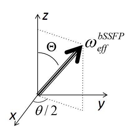
Consider only 1 pool first. In a bSSFP sequence, 5 if the relaxation is ignored, $$M_{n+1}=R_z(\theta)R_x(\alpha)M_n=R_{\overrightarrow{e}}(\Phi)M_n=e^{H_{eff}TR}M_n~~~~(1)$$where $$$M_{n+1}$$$ and $$$M_{n}$$$ are the magnetization vectors at the end of $$$n+1$$$ and $$$n$$$ cycle. $$$R_z(\theta)$$$ and $$$R_x(\alpha) $$$ are the standard z- and x-rotation matrices respectively, where $$$\theta=2\pi\Delta{TR}$$$ is the precession angle during TR and $$$\Delta$$$ is the off-resonance shift. According to the Euler theorem, $$$R_z(\theta)R_x(\alpha)$$$ can be represented by a single rotation $$$R_{\overrightarrow{e}}(\Phi)$$$, where $$$\overrightarrow{e}$$$ is the directionality vector and $$$\Phi$$$ is the rotation angle about $$$\overrightarrow{e}$$$. The effective field (Fig.1) is in the same direction as $$$\overrightarrow{e}$$$ and with the magnitude $$$\omega_{eff}^{bSSFP}$$$: $$\omega_{eff}^{bSSFP}=\Phi/TR~~~~(2)$$The $$$e^{H_{eff}TR}$$$ is the matrix exponential form of $$$R_{\overrightarrow{e}}(\Phi)$$$.
When relaxation is included, Eq.1 becomes: $$ M_{n+1}=e^{(H_{eff}-\widetilde{R})TR}M_n-[I-e^{(H_{eff}-\widetilde{R})TR}](H_{eff}-\widetilde{R})^{-1}R_1M_0~~~(3)$$where $$$\widetilde{R}=diag(R_2,R_2,R_1)$$$ is the standard relaxation matrix and $$$M_0=[0,0,M_{0}]^T$$$. From Eq.3, the steady-state magnetization $$$M_{ss}$$$ can be obtained: $$M_{ss}=-(H_{eff}-\widetilde{R})^{-1}R_1M_0~~~(4)$$ $$$H_{eff}$$$ can be expressed in its eigenbasis as $$$H_{eff}=D\Lambda_{eff}D^{-1}$$$ where $$$D$$$ is the diagonalization matrix and $$$\Lambda_{eff}$$$ is the eigenvalue diagonal matrix. $$$\widetilde{R}$$$ can also be diagonalized in the eigenbasis of $$$H_{eff}$$$, which yields $$$\widetilde{R}=D\Lambda_{R}D^{-1}$$$ where $$$\Lambda_{R}=diag(R_{1\rho},R_{2\rho},R_{2\rho})$$$, $$$R_{1\rho}=cos^2(\Theta)R_1+sin^2(\Theta)R_2$$$, $$$R_{2\rho}=sin^2(\Theta)R_1+cos^2(\Theta)R_2$$$, and $$$\Theta$$$ is the angle between the effective field and the Z-axis (Fig.1). Using the eigensystem of $$$H_{eff}$$$, the $$$M_{ss}$$$ becomes: $$M_{ss}=-D\Lambda^{-1}D^{-1}R_1M_0~~~(5)$$where $$$\Lambda=\Lambda_{eff}-\Lambda_{R}$$$.
Furthermore, the time-dependent magnetization can be derived from Eqs.3 and 5: $$M_n=M_{ss}+De^{\Lambda{\cdot}nTR}D^{-1}(M_0-M_{ss})~~~(6)$$
Now consider 2 pools, water and solute, coupled by exchange. When exchange exists, an additional term $$$R_{ex}$$$ is introduced to the water via $$$R_{1\rho}$$$ and $$$R_{2\rho}$$$: $$$R_{1\rho,w}=cos^2(\Theta_w)R_{1w}+sin^2(\Theta_w)(R_{2w}+R_{ex})$$$ and $$$R_{2\rho,w}=sin^2(\Theta_w)R_{1w}+cos^2(\Theta_w)(R_{2w}+R_{ex})$$$. Here we follow Trott and Palmer’s work 6 for $$$R_{ex}$$$ (asymmetric population limit): $$R_{ex}=\frac{p_wp_s\Delta_{ws}^2k}{(w_{eff,s}^{bSSFP}/2\pi)^2+k^2}=\frac{p_wp_s\Delta_{ws}^2k}{\Phi_s^2/(2\pi{TR})^2+k^2}~~~(7)$$where $$$p_w=M_{0w}/(M_{0w}+M_{0s})$$$, $$$p_s=M_{0s}/(M_{0w}+M_{0s})$$$, $$$\Delta_{ws}$$$ is the chemical shift between water and solute, and $$$k=k_{sw}+k_{ws}$$$, $$$k_{sw}$$$ and $$$k_{ws}$$$ are exchange rates from solute to the water pool and vice-versa.
Methods
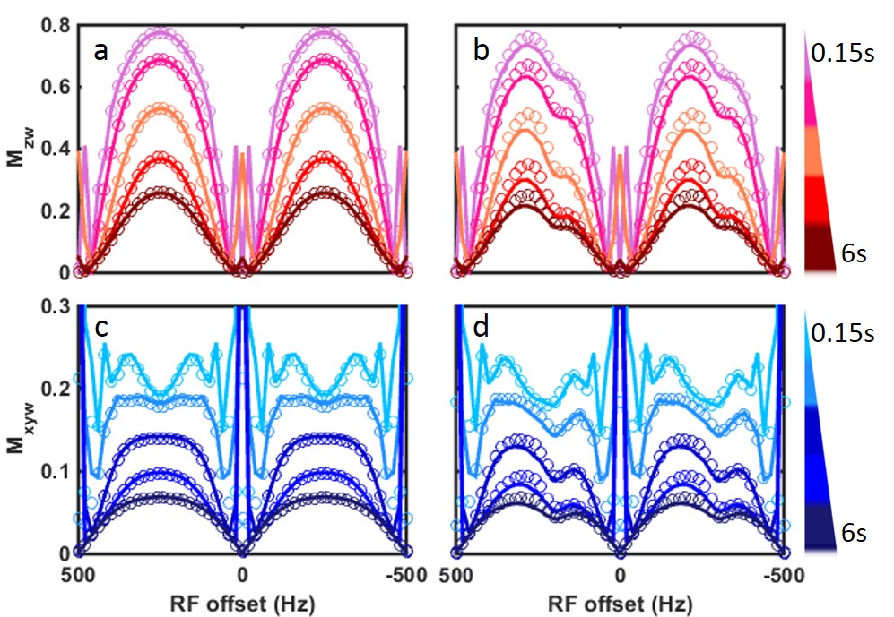
Simulations were performed using two models: a 1-pool model with M0w=1, T1w/T2w=2/0.05s and a 2-pool model with M0w=1, T1w/T2w=2/0.05s, M0s=0.005, T1s/T2s=1/1s, ∆ws=1ppm, ksw=100Hz. For all the simulations, rectangular pulses with duration 25μs, α=30o and TR=2ms were used. The magnetizations were calculated for each TR for total saturation time tsat=10s (5 times of T1w or 5T1w). To show the time evolution of the Z- and XY-spectrum, the spectra with tsat=3T2w, 5T2w, 0.25T1w, 0.5T1w and 3T1w were plotted.Results and Discussion
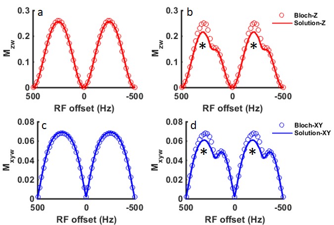
Fig.2 compares the steady-state spectra obtained using the analytical solution with the exact BME simulations. Fig.3 shows the time evolution of the Z- and XY-spectra. The analytical solution is in excellent agreement with BME for both Z- and XY-spectrum for the 1-pool model.
For the exchanging 2-pools, the solution is in good qualitative agreement with BME. At the steady-state, the solution follows BME for the most part but deviates slightly downward at the star labeled frequencies close to water (Fig.2b,d). In Fig.3, the overall behavior and the agreement at both short and long tsat is excellent, indicating that the solution correctly depicts transient oscillations with T2ρ and T1ρ relaxations. However, large deviations were observed close to the saturation bands for short tsat (tsat<3T1w). These results indicate that the exchange contribution (Eq.7) needs to be further improved.
Conclusion
In the abstract, an analytical solution to the BME is derived for bSSFPX based on the effective field. Overall, this solution is in good agreement with BME and follows the transient signal oscillations well. Deviations observed in the regions close to saturation bands at short tsat and at star labelled frequencies (Fig.2b,d *) in the 2-pool model indicate that the exchange contribution needs to be further improved. Work is in progress to use this solution to quantify the exchange rate experimentally.Acknowledgements
No acknowledgement found.References
1. Zhang S, Zheng L, Lenkinski RE, et al. in: Proc Intl Soc Mag Reson Med. 2015;23:0785.
2. Zhang S, Lenkinski RE, Vinogradov E. in: Proc Intl Soc Mag Reson Med. 2016;0304.
3. McMahon MT, Gilad AA, Zhou J, et al. Quantifying exchange rates in chemical exchange saturation transfer agents using the saturation time and saturation power dependencies of the magnetization transfer effect on the magnetic resonance imaging signal (QUEST and QUESP): pH calibration for poly-L-lysine and a starburst dendrimer. Magn Reson Med. 2006;55(4):836-847.
4. Zaiss M, Bachert P. Chemical exchange saturation transfer (CEST) and MR Z-spectroscopy in vivo: a review of theoretical approaches and methods. Phys Med Biol. 2013;58:R221-R269.
5. Freeman R, Hill H. Phase and intensity anomalies in Fourier transform NMR. J Magn Reson (1969). 1971;4(3):366-383.
6. Trott O, Palmer III AG. R1ρ Relaxation outside of the Fast-Exchange Limit. J Magn Reson. 2002;154:157-160.
Figures