Synopsis

Hypoxia is an important prognostic indicator in most solid tumours. We present here automated, data-driven methods, using principal component analysis (PCA) and Gaussian mixture modelling (GMM), that consistently locate functionally distinct sub-regions in preclinical tumours, some of which are postulated to be relevant to hypoxia. Methods are based on dynamic contrast-enhanced (DCE)-MRI (reflecting perfusion) and oxygen-enhanced (OE)-MRI (reflecting oxygen delivery). We demonstrate the utility and stability of our methods through a combination of evaluation metrics, which may be incorporated in similar studies elsewhere.

Introduction

Methods

1. Imaging

9 U87 (glioblastoma) and 7 Calu6 (non small cell lung carcinoma) xenografts were grown in the lower midline of the back of nude mice. Each mouse underwent OE-MRI followed by DCE-MRI on a 7 T Bruker system, while anaesthetised with 2% isoflurane carried initially in medical air (21% oxygen). OE-MRI consisted of a variable flip angle (VFA) spoiled gradient echo (SPGR) acquisition to calculate native tissue $$$T_1$$$ ($$$T_{10}$$$), followed by 42 dynamic $$$T_1$$$-weighted SPGR acquisitions at a temporal resolution of 28.8 s, during which the gas supply, administered via a nose cone, was switched from air to pure oxygen at acquisition 19. DCE-MRI consisted of a VFA sequence again to calculate tissue $$$T_{10}$$$ values, followed by 96 dynamic $$$T_1$$$-weighted SPGR acquisitions at a temporal resolution of 5.78 s, during which Gd-DOTA was injected into a tail vein at acquisition 25.

2. Processing

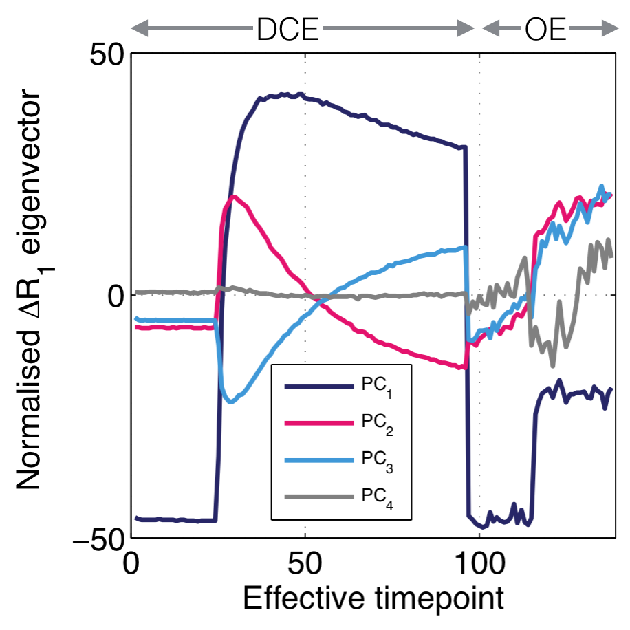
OE and DCE signals were converted to $$$\Delta R_1$$$ (change from native $$$R_1$$$ where $$$R_1 = \frac{1}{T_1}$$$) and corrected for baseline drift. OE $$$\Delta R_1$$$ values were then scaled so the standard deviation across all voxels’ time series matched that of the DCE data. Features were then extracted using PCA on concatenated DCE-OE $$$\Delta R_1$$$ time course data across all 16 animals’ tumour voxels.

3. Clustering

Prominent clusters in the PCA-derived feature set were located using GMM, with the number of clusters ($$$N_C$$$) varying from 2-25. For each $$$N_C$$$ value, mean within-cluster DCE and OE curves were calculated, and cluster assignments transferred into image space to create tumour region maps.

4. Evaluation

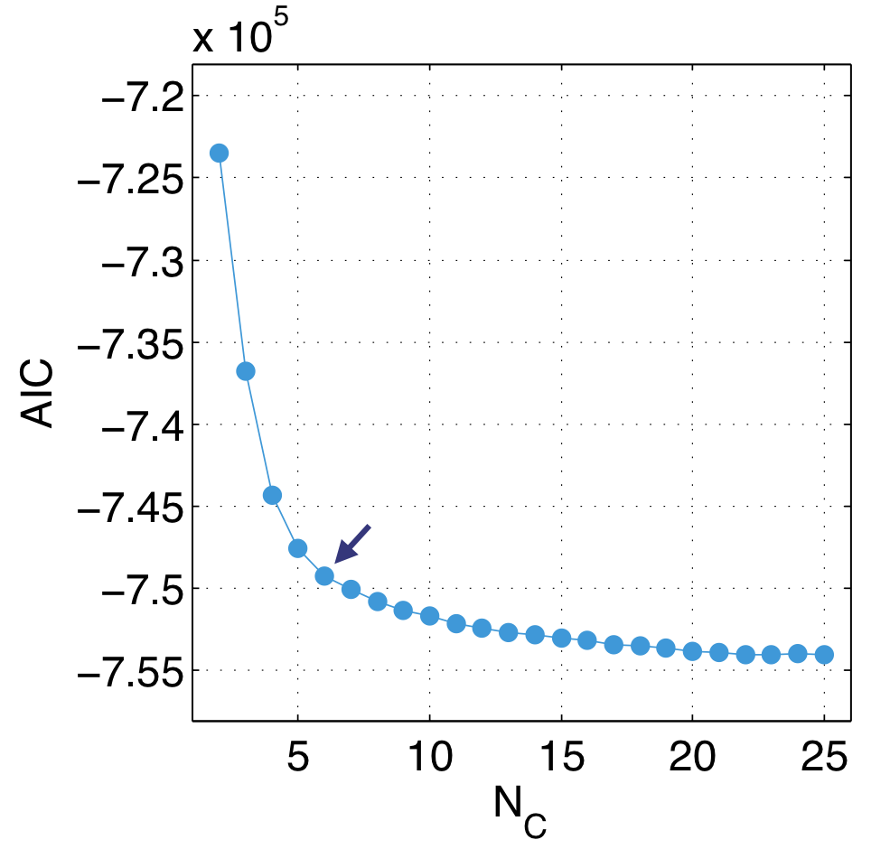
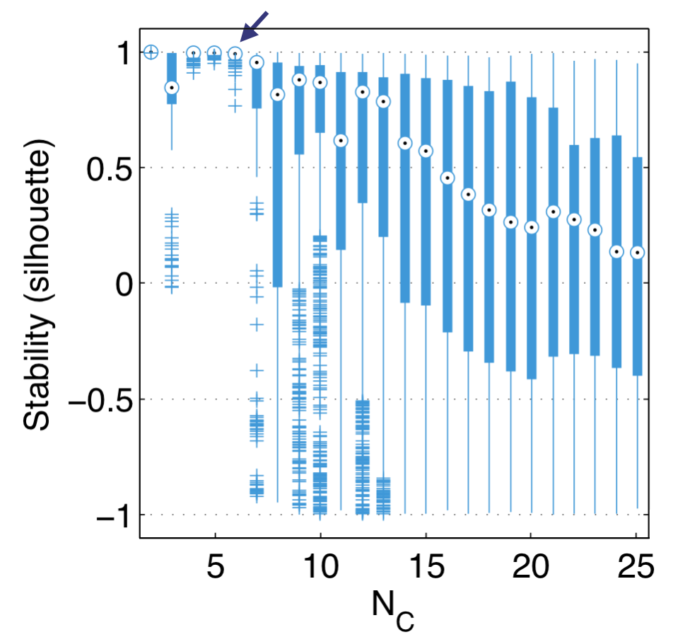
For each $$$N_C$$$, the Akaike information criterion ($$$AIC$$$) was calculated. Technique efficacy was investigated by comparing measures of regional contiguity within region maps to null distributions of contiguity generated using random resampling, and calculating contiguity z-scores. Methodological stability was assessed using bootstrap resampling of the feature distribution and quantifying the stability of the location of cluster centres across bootstrap realisations using silhouettes^[5].

Results

PCA identifies distinct kinetics of enhancement from the group of tumours, as shown in Fig. 1, with the first four principal components explaining over $$$99\%$$$ of the variance within the data set. This provided us with justification for choosing a four-dimensional feature set.

Upon clustering the feature set using GMM, we observe decreasing improvements in GMM fit quality, as assed using $$$AIC$$$, above $$$N_C = 6$$$ (Fig. 2) and we see that GMM performs robustly only when $$$N_C \leq 6$$$, when using silhouettes (Fig. 3). Contiguity z-scores remained high ($$$>3$$$) for nearly all tumours for all $$$N_C$$$. These results led us to select $$$N_C = 6$$$ as the recommended value for this data set.

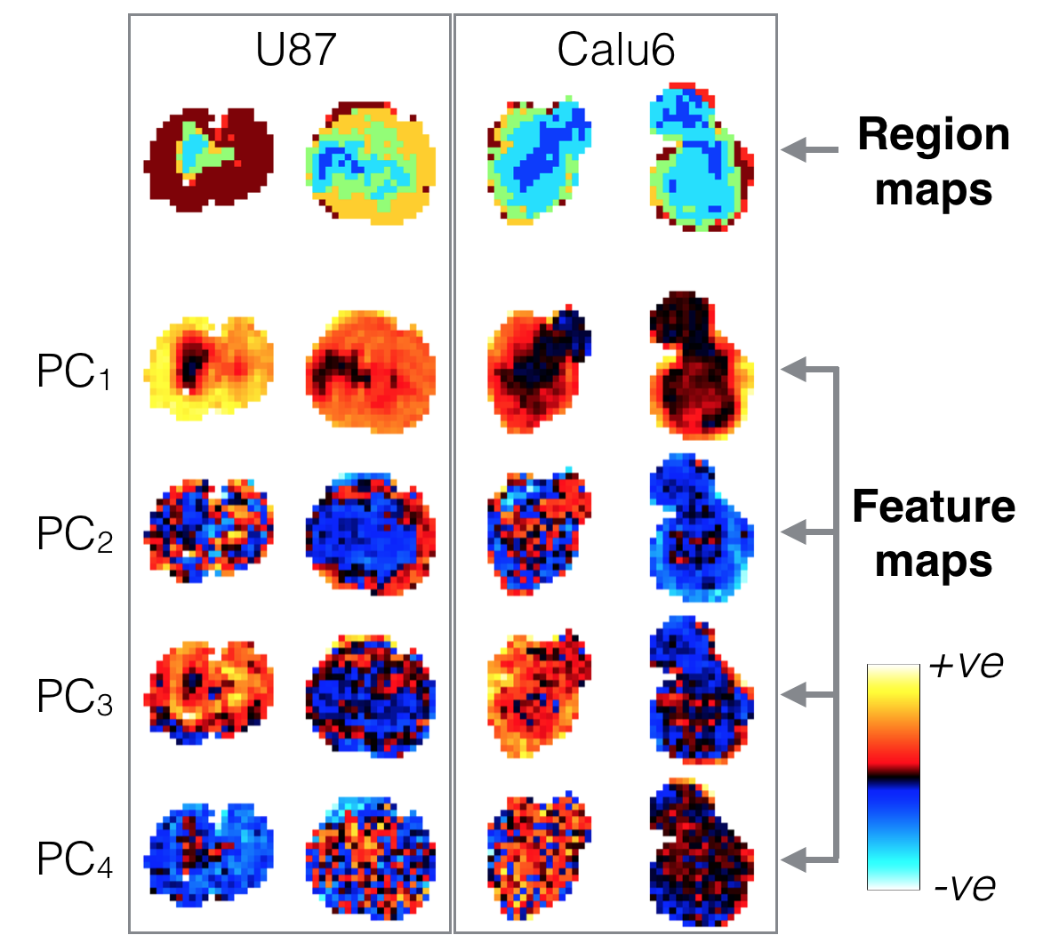
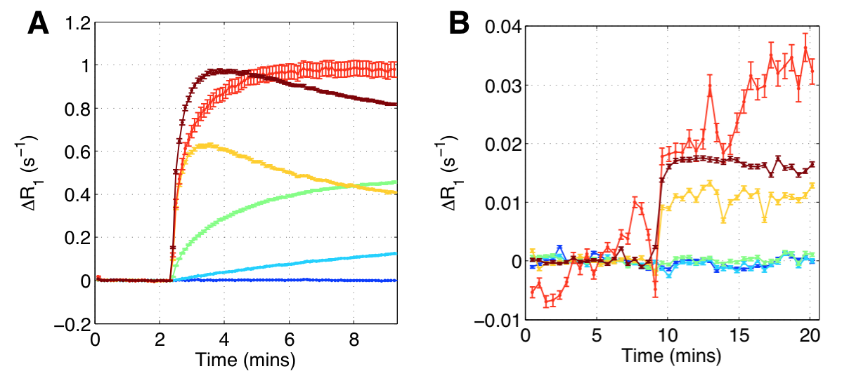
Fig. 4 shows tumour region maps from our recommended method for four representative tumours, alongside principal component feature maps. Region maps show spatially contiguous regions and a rim-core structure. Mean within-cluster enhancement curves in Fig. 5 show that GMM locates regions with distinct physiological characteristics, and with enhancement kinetics that are consistent with DCE-MRI and OE-MRI curves previously reported using manual region selection.^[3,4]

Discussion

The rim-core structures present in region maps and the high contiguity z-scores, particularly with high $$$N_C$$$ values, suggest there is a biological basis to the regions identified. The recommended method locates regions where there is DCE-MRI but not OE-MRI enhancement (green and light blue regions/curves in figures 4 and 5). These have been shown to be relevant to hypoxia.^[3,4] It is encouraging that in our current work, using a purely objective and data-driven methodology, we identify regions with these characteristics, removing the need for operator-based feature extraction.

When clustering data, we desire a high enough $$$N_C$$$ to identify features of potential importance (and in this case to adequately characterise tumour heterogeneity), whilst keeping a low enough $$$N_C$$$ to ensure the repeatability and reliability of our results. This lends importance to the range of evaluation metrics used in this study as they provide objective measures from which the optimal $$$N_C$$$ can be determined.

Conclusion

Acknowledgements

References

1: Alizadeh A A, et al. Toward understanding and exploiting tumor heterogeneity. Nat Med. 2015;21(8):846-53.

2: O’Connor J P B, et al. Imaging intratumor heterogeneity: role in therapy response, resistance, and clinical outcome. Clin Cancer Res. 2015;21(2):249-57.

3: Linnik I V, et al. Noninvasive tumor hypoxia measurement using magnetic resonance imaging in murine U87 glioma xenografts and in patients with glioblastoma. Magn Reson Med. 2014;71(5):1854-62.

4: O’Connor J P B, et al. Oxygen-enhanced MRI accurately identifies, quantifies, and maps tumor hypoxia in preclinical cancer models. Cancer Res. 2016;76(4):1-9.

5: Rousseeuw P J. Silhouettes: a graphical aid to the interpretation and validation of cluster analysis. J Comput Appl Math. 1987;20:53-65