0960
A novel method for extracting hierarchical subnetworks based on a multi-subject spectral clustering approach1Florey Institute of Neuroscience and Mental Health, Melbourne, Australia
Synopsis
Brain-network has an intrinsic hierarchical structure, which, however, cannot be uncovered using the current methods exclusively for modularity analysis. A recent study has investigated hierarchical structure of brain-network using a hierarchical-clustering approach, which, nevertheless, has the following issues: (i) it relies on applying somewhat arbitrary thresholds to cross-coefficients (different thresholds likely yield distinct clustering outcomes); (ii) individual-level clustering results at early steps are likely to introduce biases at later stages, compromising the final clustering. We propose a method, Network Hierarchical Clustering (NetHiClus), based on a multi-subject spectral-clustering approach, which can robustly identify functional sub-networks at hierarchical-level, without thresholding the cross-coefficients.
Purpose
Modularity of brain-networks provides selective adaptability, which plays a key role in developmental optimization1. Methods for analyzing modularity have already been developed2,3. Importantly, brain-network has an intrinsic hierarchical structure4. However, such hierarchical network structure cannot be uncovered using the modularity methods. A recent study investigated hierarchical-clustering, which, however, relied on applying somewhat arbitrary thresholds to cross-coefficients4; different thresholds likely yield distinct clustering outcomes. We propose a method, Network Hierarchical Clustering (NetHiClus), to robustly identify functional subnetworks at hierarchical-level, without thresholding the cross-coefficients.Methods
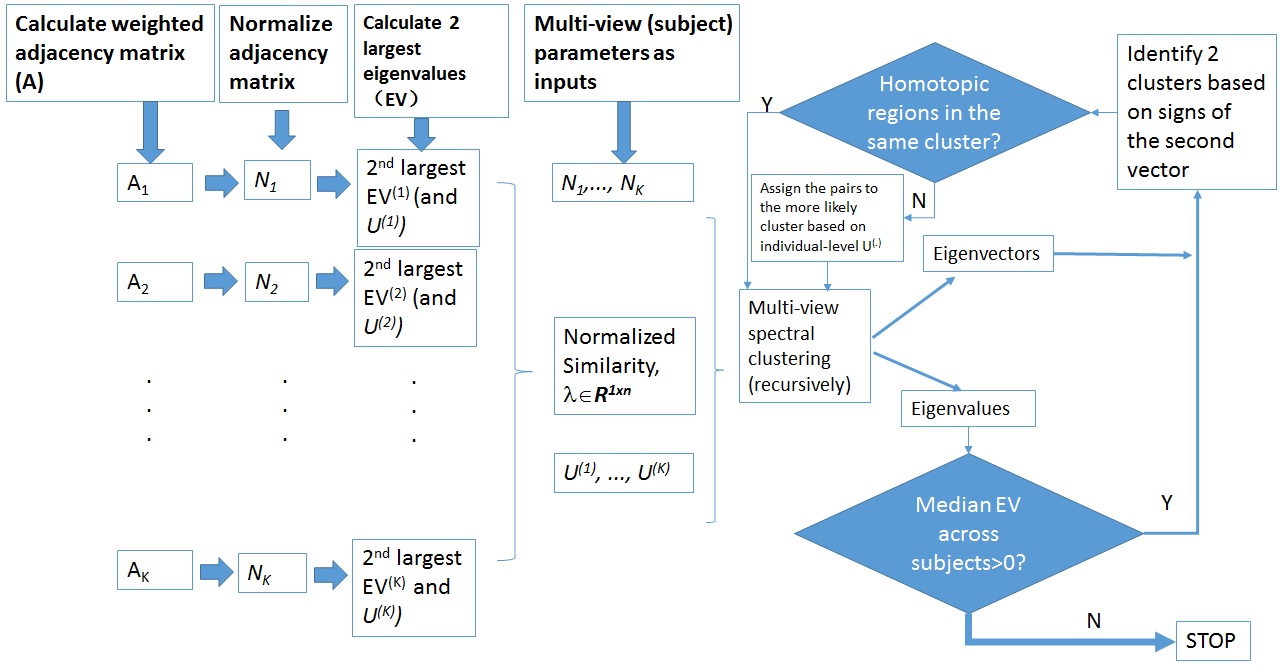
NetHiClus consists of 2 parts (part I&II) - a flowchart is shown in Figure 1:
(I) The multi-subject spectral clustering5 is used to estimate consensus (group-level) eigenvector of normalized adjacency-matrices and more consistent individual-level eigenvectors and eigenvalues across the group. It includes the following steps:
(a) Using BOLD data to calculate adjacency-matrix A(v) for subject v (v=1,...,K), with K the number of subjects in group.
(b) Calculating normalized adjacency-matrix $$$N_1^{(v)}={D^{(v)}}^{(-1/2)}A^{(v)}{D^{(v)}}^{(-1/2)}$$$, D – degree-matrix. $$$N=(N_1+N_1^{T})/2$$$ is certainly symmetric.
(c) Calculating initial eigenvectors $$$U^{(v)}$$$ by eigenvalue-decomposition of $$$N^{(v)}$$$ . We are interested in the second eigenvalue/eigenvector (see (h) below).
(d) Updating group consensus $$$U^G$$$ : solving $$$ \max \limits_{U^G \in R^{n×k}} trace\{{U^G}^T(\sum_vλ_v(U^{(v)}{U^{(v)}}^T))U^G\}$$$, $$$s.t. {U^G}^TU^G=I$$$ by eigenvalue-decomposition on $$$\sum_vλ_v(U^{(v)}{U^{(v)}}^T)$$$ , with $$$U^{(v)}$$$ from (c) for first iteration, n: #nodes, k: #clusters, $$$λ_v$$$ : weight (i.e. ‘importance’) of subject v [5] (Note: k=2 for bi-clustering in our study).
(e) Updating $$$U^{(v)}$$$ : solving $$$ \max \limits_{U^{(v)} \in R^{n×k}} trace\{{U^{(v)}}^T(N^{(v)}+λ_vU^G{U^G}^T))U^{(v)}\}$$$, $$$s.t. {U^{(v)}}^TU^{(v)}=I$$$, by eigenvalue-decomposition on with all other $$$U^{(v)}$$$ and $$$U^G$$$ fixed5.
(f) Updating $$$U^{(v)}$$$ and $$$U^G$$$ iteratively via (d) and (e) until convergence5, yielding final estimates of $$$U^G$$$ ,$$$U^{(v)}$$$ and $$$EV^{(v)}$$$ (eigenvalues).
(II) The hierarchical-clustering is used to hierarchically divide the networks into 2 clusters using $$$U^G$$$, $$$U^{(v)}$$$ and $$$EV^{(v)}$$$ from (I).
(g) For each cluster, if the median of second largest eigenvalues of individual subject ($$$U^{(v)}$$$) across the group is positive, go to step (h); otherwise stop3;
(h) The vector corresponding to the second largest eigenvalue (i.e. Fiedler vector) is employed to assign the nodes into 2 different clusters based on their signs (i.e. “+” vs. “-”)6.
(i) Furthermore, since brain sub-networks tend to be bilateral4, homotopic brain regions are forced to be present in the same sub-networks to which the homotopic regions are more likely belonging.
(j) The 2 new clusters obtained at the current-level are fed into (I) recursively.
MRI data: Resting-state HCP (www.humanconnectomeproject.org) FIX-denoised fMRI data (n=133) were used: TR/TE=700/33.1ms, 2mm isotropic, 1200 volumes.
Data analyses: Network construction: (i) AAL-atlas is used to parcellate the whole-brain into 90 regions; (ii) a mean time-series is calculated in each region; (iii) connectivity is obtained using Pearson-correlation.
Clustering evaluation
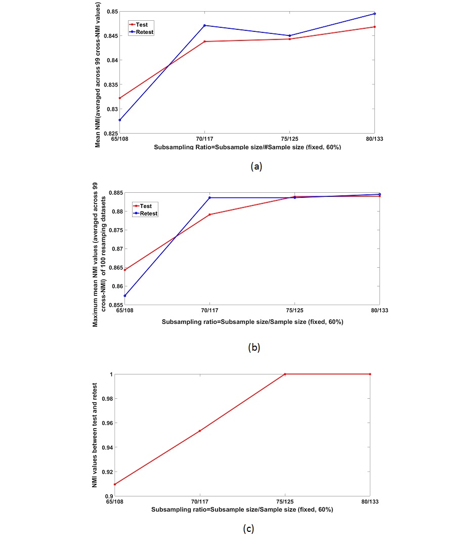
(i) Robustness: (a) 100 random subsamples were generated for each of 4 subsampling cases (fixed ratio=60%, but with variable subsampling size: $$$65/108,70/117,75/125/80/133$$$ ); (b) NetHiClus was applied to each case; (c) normalized mutual information (NMI)7 was calculated between each subsample and the remaining 99 subsamples (cross-NMI), yielding mean cross-NMI (CN) for each subsample; (d) the subsample having the maximum CN was designated as the one obtaining the most reliable clustering results from the 100 subsamples.
(ii) Reproducibility: two groups of subsamples were generated for each case to evaluate the test-retest reliability.
Results
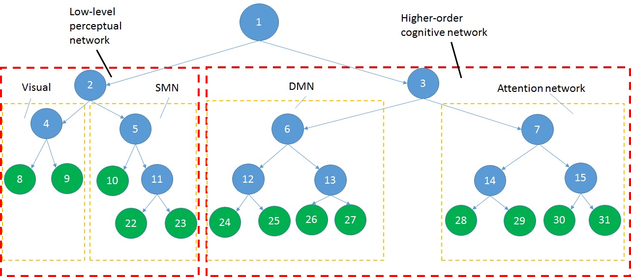
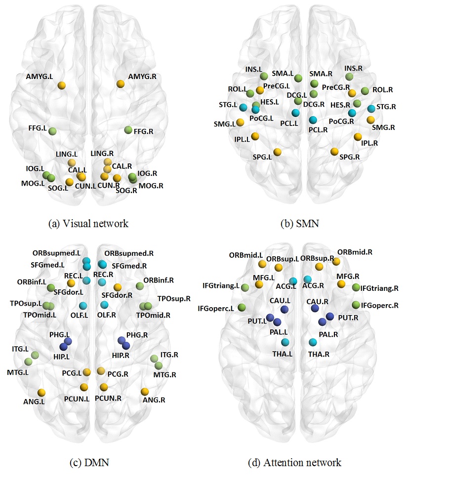
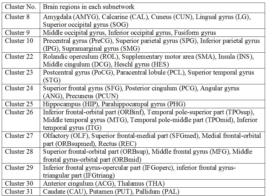
Figure 2 shows 13 functional subnetworks of the human brain found using NetHiClus. Networks are first divided into low-level perceptual and high-level cognitive networks, from which well-known networks are clustered hierarchically. These include visual, somato-motor, default-mode, and attention networks, with specific brain regions listed in Table 1. Each of these networks is mapped onto the AAL-atlas; each network is then hierarchically clustered into indivisible subnetworks, with each subnetwork represented in a different color (Figure 3). Test-retest experiments demonstrate that (i) larger subsample size leads to higher reproducibility (Figure 4); (ii) exactly consistent clustering results can be achieved at sample-size >75 (Figure 4(c)). However, 6 and 3 regions (averaged across test and retest) were incorrectly clustered for 65/108 and 70/117.Discussion
We propose a method, NetHiClus, for hierarchically clustering the brain-network into subnetworks, without relying on applying arbitrary thresholds to cross-coefficients, as previously done4. Importantly, rather than performing clustering at individual-level, we tackle this problem using a multi-subject approach, sharing information across subjects. Our results show that NetHiClus can hierarchically cluster functional network into specialized subnetworks, fulfilling specialized tasks; conversely, information processed by specialized inferior-level subnetworks are integrated into superior-level for achieving optimal efficiency. Importantly, test-retest results have demonstrated the robustness of NetHiClus. Our findings are consistent with the concept of network segregation and integration8. This should promote the understanding of brain network from a hierarchical point of view.
Acknowledgements
No acknowledgement found.References
1. Simon H. 1962. The architecture of complexity. Proc. Am. Philos. Soc. 106, 467–482.
2. Newman M.E.J. 2006. Modularity and community structure in networks. PNAS 103: 8577-82.
3. Newman M.E.J., Girvan M., 2004. Finding and evaluating community structure in networks. Phys. Rev. E 69: 026113.
4. Meunier D., Lambiotte R., Fornito A. 2009. Hierarchical Modularity in human brain functional networks. Front Neuroinformatics, 3:37.
5. Kumar A., Rai P., Daume III, H. 2011. Co-regularized multi-view spectral clustering. Proceedings of the 24th International Conference on Neural Information Processing Systems. 1413-21.
6. Fiedler, M. 1973. Algebraic connectivity of graphs. Czechoslovak Math. J., 23:298:305.
7. Lancichinetti A., Fortunato S., Kertesz J. 2009. Detecting the overlapping and hierarchical community structure in complex networks. New J. Phys., 11(3): 033015+.
8. Sporns O. 2013. Structure and function of complex brain networks. Dialogues Clin Neurosci, 15(3): 247-62.
Figures