0954

A simple data driven predictive dynamical model of whole brain resting state fMRI signal behavior

Eric Wong¹

¹Radiology/Psychiatry, UC San Diego, La Jolla, CA, United States

Synopsis

In this work we present a simple dynamical model that learns from resting state fMRI data to predict future brain states using information from one or more past brain states. We use a fully connected neural network model, and data from the Human Connectome Project. Our group model explains over 45% of the variance across 472 subjects, is very consistent when trained on subsets of the subjects, predicts realistic dynamics, gravitates towards the default mode when started in nearly any simulated brain state, and is complementary to correlation analysis.

Introduction

Resting state fMRI data is most commonly analyzed using correlation as a metric of connectivity. This approach has at least two fundamental drawbacks. First, because correlations are undirected, it is difficult to utilize correlation data to construct a model of brain dynamics. Second, correlation does not imply a direct connection between areas, and may instead represent correlations through intermediate areas. In this work we present a simple dynamical model that learns from resting state fMRI data to predict future brain states using information from one or more past brain states. The goals of this work are to ask whether information that is asymmetric in time can be learned from resting state data, whether learned connections are complementary to those calculated using correlation, and whether the dynamics predicted by the model are informative.

Methods

Data: Our model was trained and tested on resting state data from the Human Connectome Project (HCP) S500 data release (1). From this group, 472 subjects were identified who had 4 complete resting state scans. Cortical grayordinate data from the HCP minimal preprocessing pipeline including MSM-All alignment were downloaded. On a per-grayordinate basis, data were demeaned, a second order polynomial was fit to and regressed out of the data, and the data were expressed as a percent change from the mean. Data were then parcellated using the HCP multi-modal parcellation (2) by taking the mean value of the grayordinate data over each parcel.

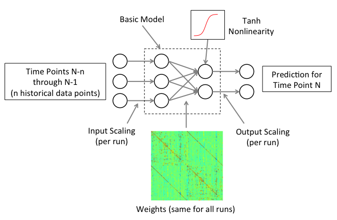
Dynamical Brain Model (Figure 1).: In our basic model, the fMRI signal in each parcel for time point T is predicted as a linear combination of the fMRI signals from all parcels at time T-1. This can be visualized as a simple fully connected neural network with one input layer and one output layer. The error signal was the difference between the prediction and the data. Weights were learned by backpropagation of these errors. Weights were learned on all data from all subjects, with each data point presented to the network 10 times. For each repetition, the order of presentation to the network was randomized over both subjects and runs.

Several variations of the basic model were tested, including: global signal regression (GSR); the addition of input and output scaling weights to account for inter-subject differences in signal scaling; a non-linear component; and the use of two or more historical time points as input to the model.

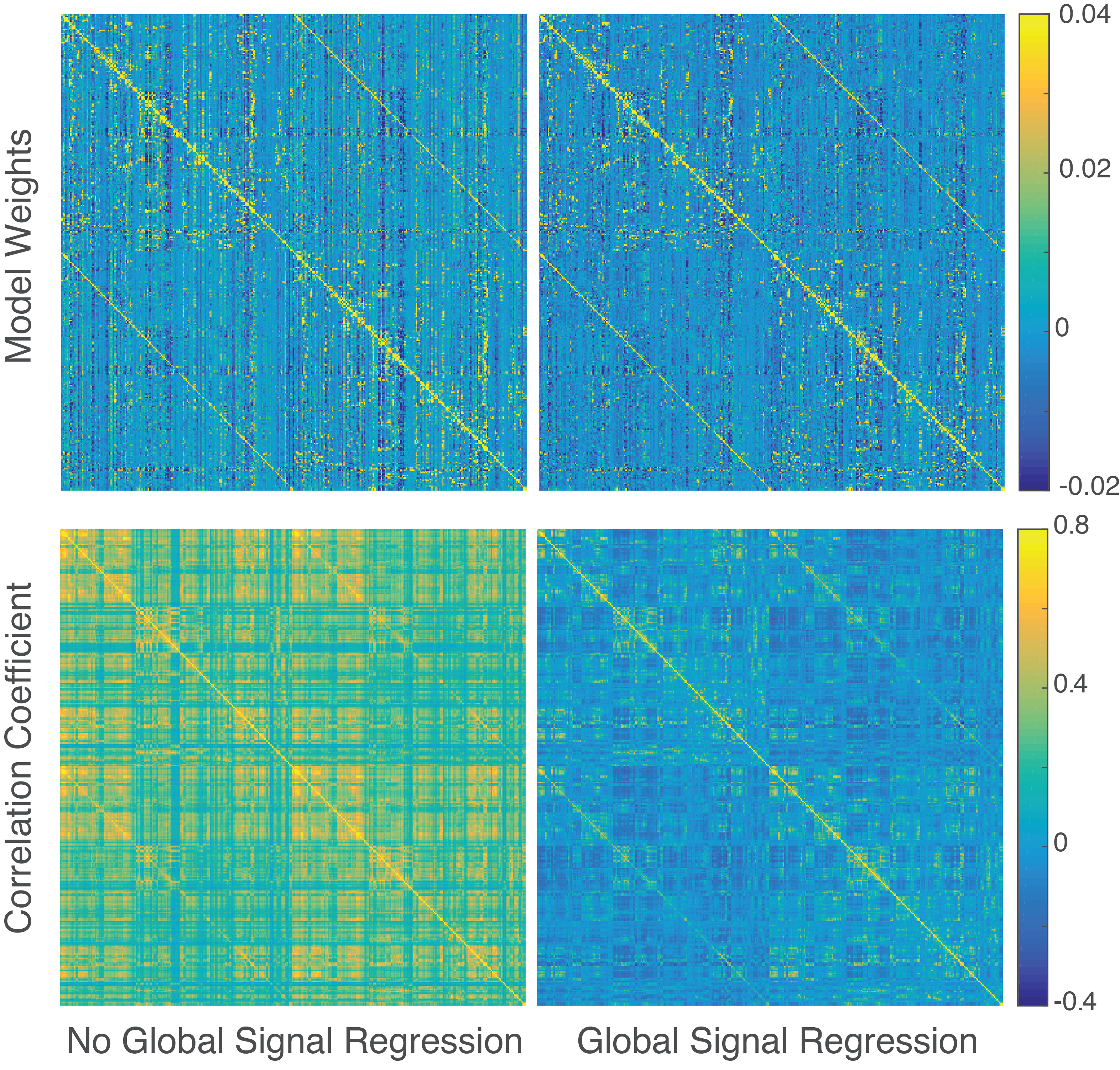
For comparison, conventional correlation analysis was performed on the same dataset by concatenating the data in time across all subjects and runs, and calculating the correlation coefficient between every pair of parcels.

Results

Figure 2 shows the model weights learned using the basic model on all 472 subjects, the correlation matrix for the same data, and the effects of GSR on each. The vertical streaks in the weight matrix that are attenuated by GSR can be interpreted as indicating parcels that have a strong tendency to trigger global signal changes in the future, and are well preserved across subsets of subjects.

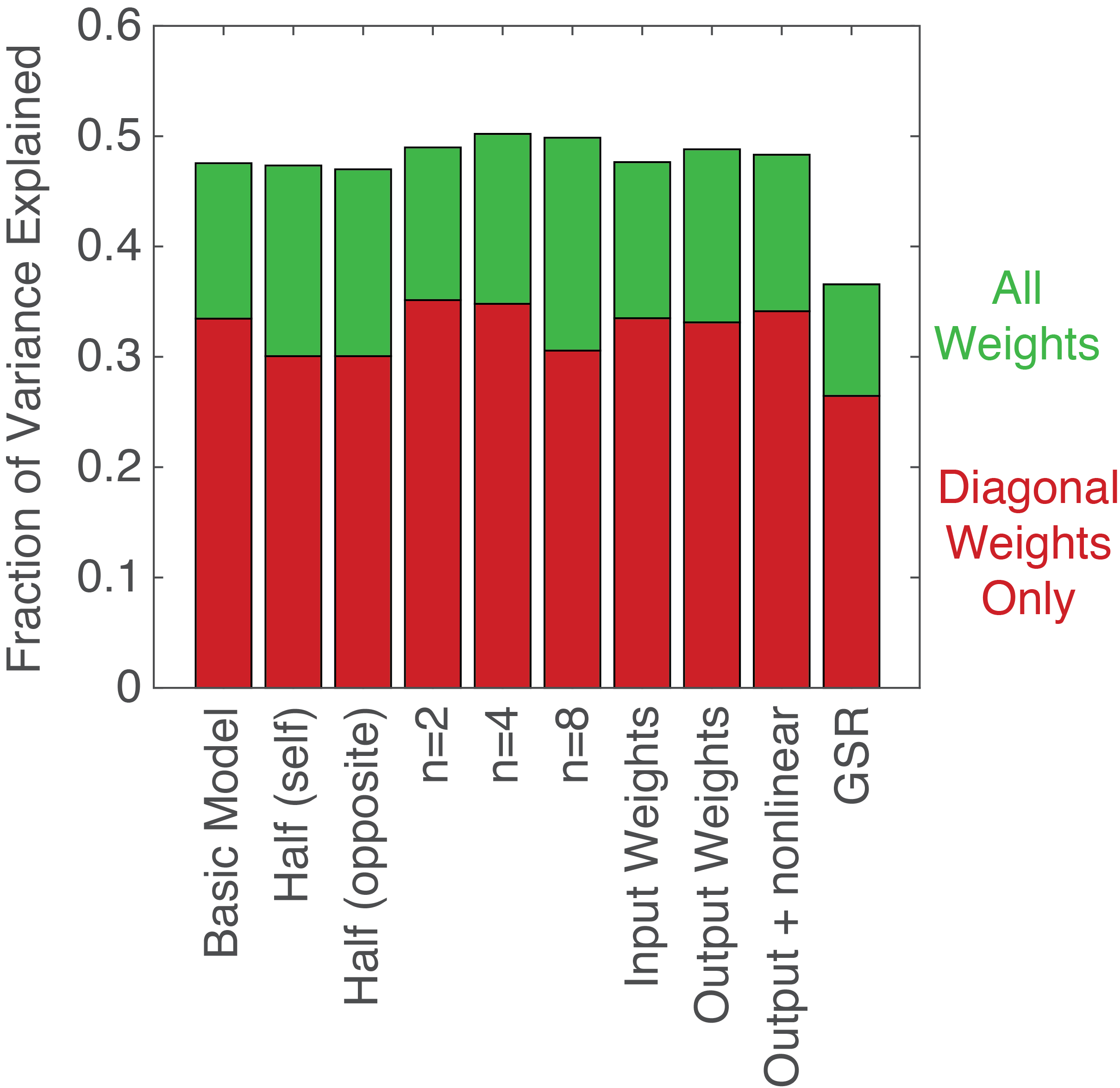
Figure 3 shows the fraction of the total signal variance explained by our model (see caption). Weights learned separately from two halves of the subject pool were nearly identical, with a correlation of 0.96. Weights trained on one half of the subjects predicted the signal dynamics of the other half of the subjects nearly as well as their own. The addition of additional historical time points, input weights, output weights, and non-linearity had minimal effect. With GSR, the fractional variance explained was decreased. However, the absolute residual variance was 13% lower than without GSR.

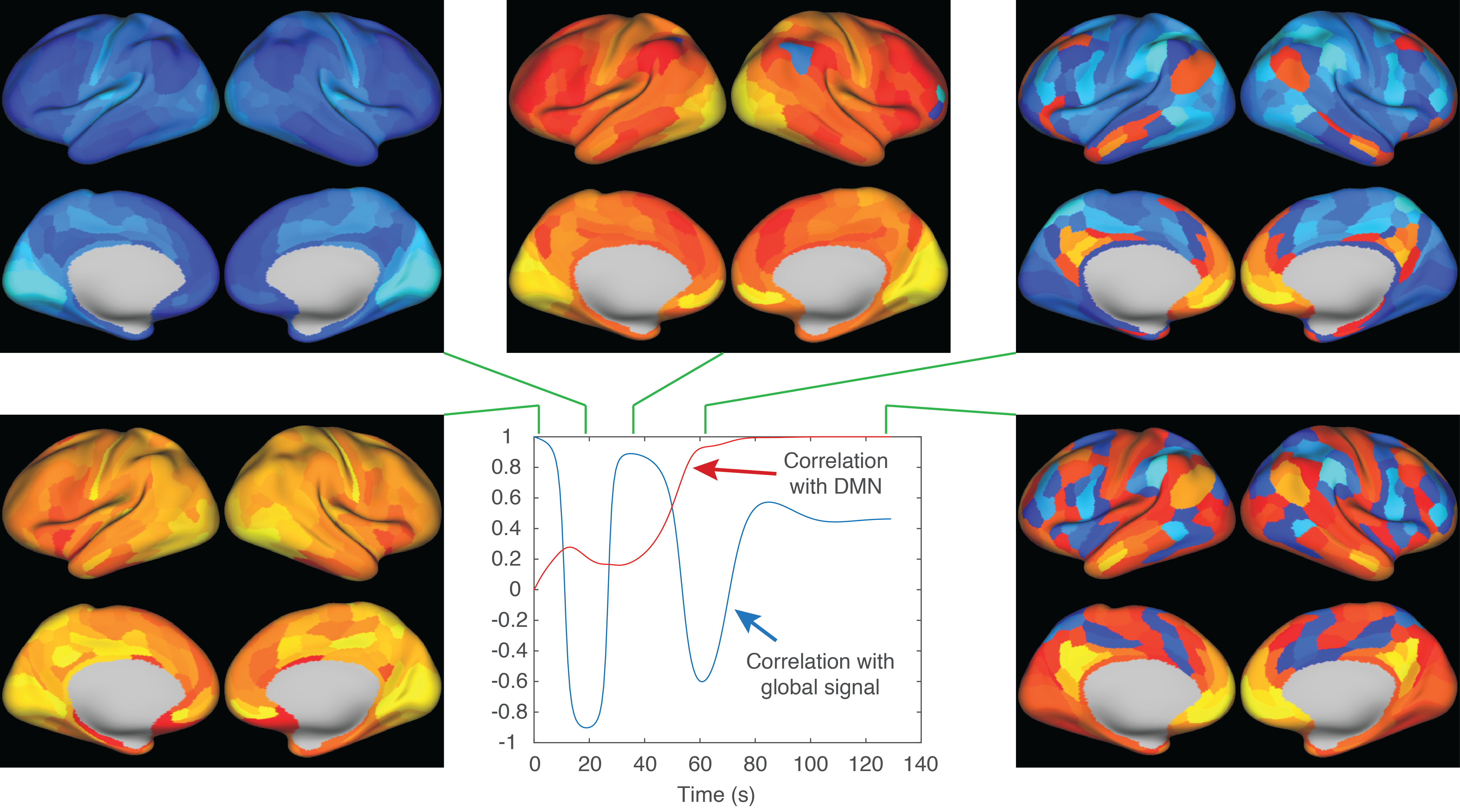
Figure 4 shows dynamics predicted using our model iteratively, showing global oscillations, and decay towards the default mode (see caption).

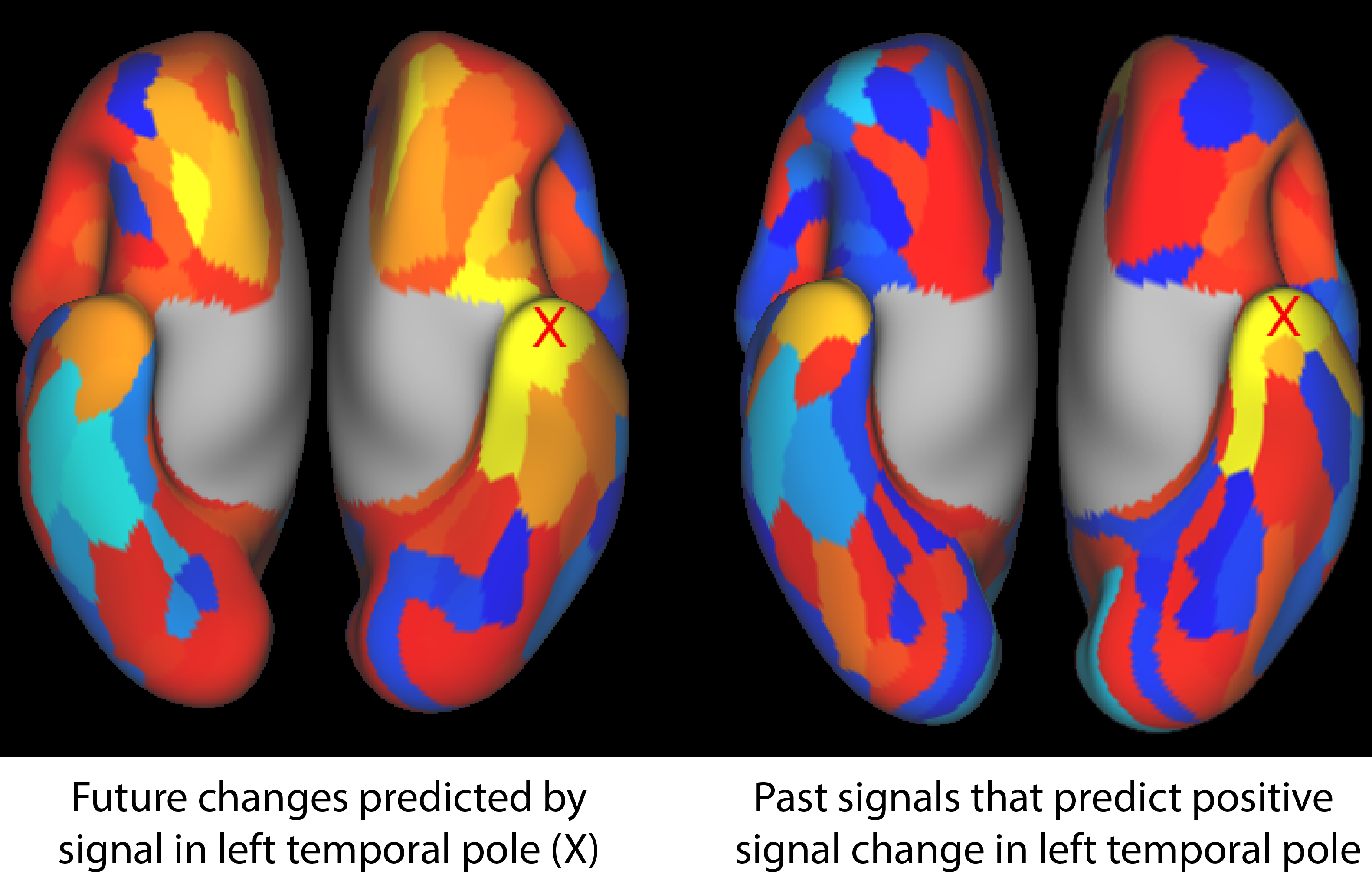
Figure 5 shows that asymmetry in time can be detected in the data using our dynamical model.

Discussion

Our dynamical model captures dependencies between parcels that are more sparse than those described by correlation. We postulate that while correlation likely overestimates the set of connected parcels because it cannot identify connections through third parties, our model likely underestimates connections because it is looking for a minimal set of parcels which can be combined to form a prediction.

Despite our model being trained on a single time step, we are encouraged that the default mode appears in dynamic forward simulations over tens of seconds, and from nearly any starting state.

We plan to extend the model to examine individual subjects, and include subcortical structures, different and per-subject parcellations, more realistic signal models, and task data with paradigm timing as inputs.

Acknowledgements

No acknowledgement found.

References

1. Matthew F. Glasser, Stamatios N. Sotiropoulos, J. Anthony Wilson, Timothy S. Coalson, Bruce Fischl, Jesper L. Andersson, Junqian Xu, Saad Jbabdi, Matthew Webster, Jonathan R. Polimeni, David C. Van Essen, and Mark Jenkinson (2013). The minimal preprocessing pipelines for the Human Connectome Project. Neuroimage 80: 105-124.

2. Glasser MF, Coalson TS, Robinson EC, Hacker CD, Harwell J, Yacoub E, Ugurbil K, Andersson J, Beckmann CF, Jenkinson M, Smith SM, Van Essen DC. A multi-modal parcellation of human cerebral cortex. Nature 2016;536(7615):171-178.

Figures

Figure 1: Schematic diagram of brain model. Basic model is a fully connected network of weights to predict future BOLD fMRI signals based on past BOLD signals. Additional features such as input and output weights, non-linearity, multiple input time points, and preprocessing with global signal regression were also tested. Weights were learned by back-propagation, and were trained on 4800 data points from each of 472 subjects in the HCP database, using the HCP MSM-All 360 parcel group parcellation.

Figure 2: Top: Learned model weights without and with GSR. Columns represent the effect of a given parcel on future signal changes across the cortex, while rows represent the dependence of the future signal in a given parcel on the past signal of all parcels. Bottom: Group correlation matrices between parcels. Peaks along diagonals within upper right and lower left quadrants represent high predictive value between corresponding parcels across hemispheres. Note that the model weights are much more sparse than the correlation matrices. Vertical lines in model weight matrices indicate parcels that tend to trigger global signals.

Figure 3: Fraction of total signal variance explained by our model. Using the basic model, nearly 50% of the total signal variance was explained by the model prediction. Approximately 2/3 of the variance explained (red bars) for each parcel was due the the past signal of the same parcel (diagonal elements of the weight matrix). The additional explained variance (green) represented the predictive value across parcels. Half (self): weights learned from one half of the subjects, explaining the same half. Half (opposite): weights learned from one half, applied to the other half. n=[2,4,8]: using n past time points for prediction.

Figure 4: Dynamics predicted by forward model. The brain was initialized in a global positive state, and the basic model was applied repeatedly to predict dynamics. The global signal oscillates with a period of approximately 40s, and the brain eventually gravitates to the default mode. This is consistent with eigenvector analysis of the weight matrix, which reveals a principal eigenvector that is identical to the default mode. The second eigenvector is a globally positive signal with emphasis on the visual cortex, as in the center image above, and has a complex eigenvalue with a rotational period of approximately 47s.

Figure 5: Asymmetry in weight matrix. Unlike correlation analysis, which can only reveal symmetrical connectivity, our dynamical model can detect dependencies that are directional in time. Shown here is column 311 (left) and row 311 (right) of the weight matrix itself. These represent, respectively, future changes predicted by a positive signal in the left temporal pole, and a map of areas that collectively predict future signal changes in the left temporal pole. While these results reveal clearly directional dependencies, they do not directly imply causality, as there may be regional differences in the timing of the underlying hemodynamic response.

Proc. Intl. Soc. Mag. Reson. Med. 25 (2017)

0954