0953

Generalized Recurrent Neural Network accommodating Dynamic Causal Modelling for functional MRI analysis

Yuan Wang¹, Yao Wang², and Yvonne W Lui³

¹Tandon School of Engineering, New York University, Brooklyn, NY, United States, ²Tandon School of Engineering, New York University, ³School of Medicine, New York University

Synopsis

We propose DCM-RNN, a new model for effective connectivity estimation from fMRI signal that links the strengths of traditional Dynamic Casual Modelling (DCM) and deep learning. It casts DCM as a generalized Recurrent Neural Network (RNN) and estimates the effective connectivity using backpropagation. It extends DCM with a more flexible framework, unique estimation methods, and neural network compatibility. In simulated experiments, we demonstrate that DCM-RNN is feasible and can be used to estimate the effective connectivity.

Introduction

Dynamic Causal Modelling (DCM) ¹ is a highly nonlinear generative model used to infer causal architecture of coupled dynamical systems in the brain from functional MRI (fMRI) data, namely, effective connectivity ². It is considered the most biologically plausible as well as the most technically advanced fMRI modeling method ^3,4. It relies primarily on variational-based methods to estimate its parameters ^5–9.

We propose to cast the DCM as a Generalized Recurrent Neural Network (GRNN) (to be called DCM-RNN) and use backpropagation based methods to estimate the causal architecture. It has the following potential advantages:

1. DCM-RNN is a more flexible framework. One can pursue model parameter sparsity and data fidelity simultaneously by specifying an appropriate loss function for network training, while these objectives have to be done separately in traditional DCM^10,11. It is also easier to add more biophysical constraints in DCM-RNN such as the sigmoid non-linearity suggested in ^12,13.

2. DCM-RNN can leverage efficient parameter estimation methods that have been developed for RNN, e.g. Truncated Backpropagation Through Time (TBPTT)¹⁴, which are significantly different from any existing methods for DCM. It circumvents some limitations of variational-based methods. For instance, it does not rely on the non-biophysically inspired Gaussian assumption about target parameters as in ^5–8. It optimizes its loss function directly, not a lower bound of the loss function as in variational-based methods.

3. DCM-RNN is biophysical meaningful and compatible with other Neural Networks (NN). Deep learning provides exciting opportunities for medical applications¹⁵. Works^16,17 have applied generic RNN in attempts to understand brain functional responses in complex tasks like movie watching. However, the generic RNNs lack biophysical interpretability. DCM-RNN can be used instead to dig more biophysical insights.

Theory

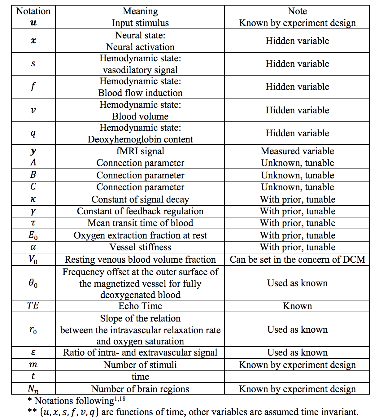
An overview of DCM is shown in Fig. 1 and the notations are summarized in TABLE I. DCM is a model for continuous time signal. The first step is to discretize it for modeling discrete time signal. Taking the neural activity state function x_t as an example. Using the approximation:

$$\mathbf{x} ̇_t≈\frac{\mathbf{x}_{t+1}-\mathbf{x}_t}{Δt}$$

where Δt is time interval between adjacent time points, the neural equation for becomes

$${\mathbf{x}_{t+1}≈(Δt\times A+I) \mathbf{x}_t+∑_{j=1}^mΔt\times u_t^{(j)} B^{(j)} \mathbf{x}_t +Δt\times C\mathbf{u}_t}$$

This trick can be applied to all the differential equations in DCM.

To accommodate the complex DCM, we propose a generalization of RNN. The classic RNN¹⁸ models inputs x_t and outputs y_t as

$$\mathbf{h}_t=f^h (W^{hx}\mathbf{x}_t+W^{hh}\mathbf{h}_{t-1}+\mathbf{b}^h )$$

$$\mathbf{y}_t=f^y (W^{yh}\mathbf{h}_t+\mathbf{b}^y )$$

where h is hidden state, W and b with various superscripts are weighting matrices and biases. f^h and f^y are nonlinear functions up to researchers’ choice and targeted applications. We generalize the classic RNN to

$$\mathbf{h}_t=f^h (W^h ϕ^h (\mathbf{x}_t,\mathbf{h}_{t-1};\mathbf{ξ}^h )+\mathbf{b}^h )$$

$$\mathbf{y}_t=f^y (W^{yh} ϕ^y (\mathbf{h}_t;\mathbf{ξ}^y )+\mathbf{b}^y )$$

The difference is the generally nonlinear functions ϕ^h and ϕ^y introduced, which are parameterized by ξ^h and ξ^y. The GRNN is trainable by backpropagation as long as ϕ^h and ϕ^y are partially differentiable. The original DCM¹ can be cast as a GRNN, as illustrated in Fig. 2, which involves three ϕ functions. We refer to the model as DCM-RNN.

We propose to infer the parameters $$$Θ=\{A,B,C,κ_n,γ_n,τ_n,{E_0}_n,α_n | n=1,2...N_n\}$$$ of DCM-RNN by using a loss function that promotes model sparsity and prediction accuracy simultaneously:

$$L(Θ)= ∑_{t=1}^T‖\mathbf{y}_t-\mathbf{y} ̂_t‖_2^2 +λ∑_{θ∈\{A,B,C\}}|θ|_1 +β∑_{n=1}^{N_n}∑_{θ∈\{κ_n,γ_n,τ_n,{E_0}_n,α_n \}}\frac{(θ-mean(θ))^2}{variance(θ)}$$

where y_t and $$$y ̂_t$$$ are the measured and estimated fMRI signal. T is the scan length. n is brain region index and N_n is total number of brain regions. λ and β are user-defined factors. The mean and variance of hemodynamic parameters come from previous studies and are listed in ¹. The loss is minimized over the whole set of Θ.

Method and Results

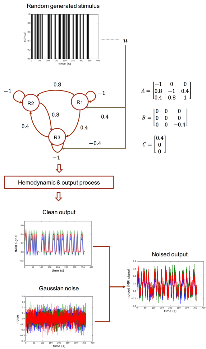
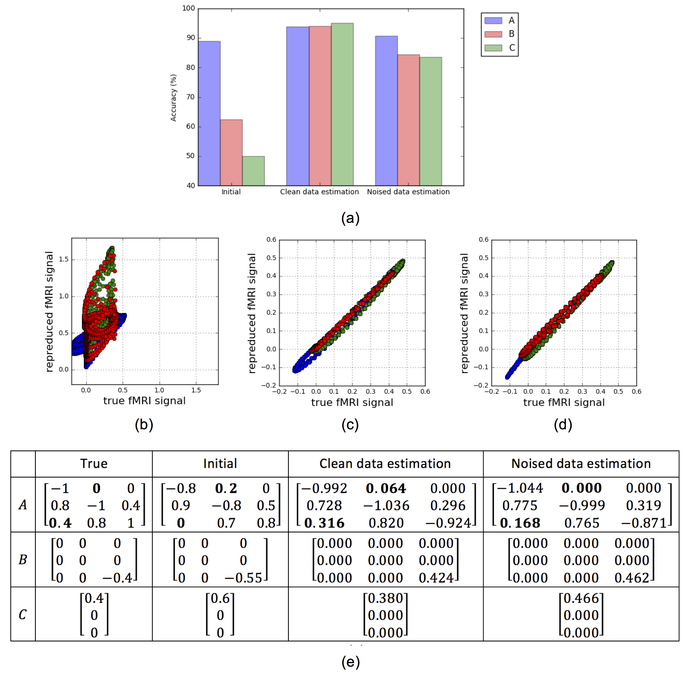
We demonstrate the feasibility of our proposal with simulated fMRI data. The data generating process is illustrated Fig. 3. Given the generated stimulus and fMRI data, we tune the DCM-RNN parameters, identifying the casual architecture, by minimizing the previously defined loss function. Experiment results are shown in Fig. 4.

Discussion

It is clear that DCM-RNN can identify the causal architecture. Besides, there are some interesting observations. First, in the initial A, the a₃₁ edge is missing and the a₁₂ edge presents falsely. In the final estimation results, such error is largely corrected: the a₃₁edge is added back and the a₁₂ edge is greatly suppressed or even removed completely. Second, the overall sparse patterns in are nicely detected and kept. It reflects the effect of l₁ sparse penalty in the loss function.

Conclusion

We have demonstrated a proof of concept for DCM-RNN, a new model for effective connectivity estimation that links the strengths of traditional DCM and deep learning.

Acknowledgements

This work was supported in part by RO1 NS039135-11 from the National Institute for Neurological Disorders and Stroke (NINDS) and was performed under the rubric of the Center for Advanced Imaging Innovation and Research (CAI2R, www.cai2r.net), a NIBIB Biomedical Technology Resource Center (NIH P41 EB017183).

We thank Quanyan Zhu, Assistant Professor, NYU, for suggestions during the development of this work.

References

1. Friston KJ, Harrison L, Penny W. Dynamic causal modelling. Neuroimage 2003; 19(4):1273–1302.

2. Friston KJ. Functional and effective connectivity: a review. Brain Connect. 2011; 1(1):13–36.

3. Smith SM. The future of FMRI connectivity. Neuroimage 2012; 62(2):1257–1266.

4. Smith SM, Vidaurre D, Beckmann CF et al. Functional connectomics from resting-state fMRI. Trends Cogn. Sci. 2013; 17(12):666–682.

5. Friston K, Mattout J, Trujillo-Barreto N et al. Variational free energy and the Laplace approximation. Neuroimage 2007; 34(1):220–234.

6. Daunizeau J, Friston KJ, Kiebel SJ. Variational Bayesian identification and prediction of stochastic nonlinear dynamic causal models. Phys. D Nonlinear Phenom. 2009; 238(21):2089–2118.

7. Friston KJ, Trujillo-Barreto N, Daunizeau J. DEM: A variational treatment of dynamic systems. Neuroimage 2008; 41(3):849–885.

8. Friston K, Stephan K, Li B, Daunizeau J. Generalised filtering. Math. Probl. Eng. 2010. doi:10.1155/2010/621670.

9. Friston KJ. Variational filtering. Neuroimage 2008; 41(3):747–766.

10. Penny WD, Stephan KE, Mechelli A, Friston KJ. Comparing dynamic causal models. Neuroimage 2004; 22(3):1157–1172.

11. Friston KJ, Li B, Daunizeau J, Stephan KE. Network discovery with DCM. Neuroimage 2011; 56(3):1202–1221.

12. Marreiros AC, Kiebel SJ, Friston KJ. Dynamic causal modelling for fMRI: A two-state model. Neuroimage 2008; 39(1):269–278.

13. Wilson HR, Cowan JD. A mathematical theory of the functional dynamics of cortical and thalamic nervous tissue. Biol. Cybern. 1973; 13(2):55–80.

14. Williams RJ, Zipser D. A Learning Algorithm for Continually Running Fully Recurrent Neural Networks. Neural Comput. 1989; 1(2):270–280.

15. Greenspan H, VanGinneken B, Summers RM. Guest Editorial Deep Learning in Medical Imaging?: Overview and Future Promise of an Exciting New Technique. IEEE Trans. Med. Imaging 2016; 35(5):1153–1159.

16. Güçlü U, van Gerven MAJ. Modeling the dynamics of human brain activity with recurrent neural networks. Front. Syst. Neurosci. 2016:1–19.

17. Qian P, Qiu X, Huang X. Bridging LSTM Architecture and the Neural Dynamics during Reading. Ijcai 2016.

18. Zachary C. Lipton. A Critical Review of Recurrent Neural Networks for Sequence Learning. arXiv Prepr. 2015:1–35.

19. Stephan KE, Weiskopf N, Drysdale PM et al. Comparing hemodynamic models with DCM. Neuroimage 2007; 38(3):387–401.

Figures

Fig. 1 A schematic overview of DCM. Edited from^1,18. Dot on a variable means its temporal derivative. Given stimuli u, neural activity x over brain regions is governed by the neural state equation. x influences vasodilatory signal s which would then trigger blood flow f change . Finally, blood volume v and deoxyhemoglobin content q determine the observable fMRI signal y. Notably, brain activities in different brain regions are coupled at neural level but not at the hemodynamic or output level. The large black-lined block means its content is repeated for each region.

TABLE 1 Variables in DCM

Fig. 2 DCM-RNN. Comparing to classic RNN, it has three extra nonlinear functions ϕ^x, ϕ^y, and ϕ^o. They are all multiple input multiple output functions. ϕ^x and ϕ^o have no parameters and ϕ^y is parameterized by α and E₀. The relationship between parameters in DCM and in DCM-RNN are clearly shown. Particularly, the matrices {A, B, C} in DCM are embedded in matrices {W^xx, W^xxu, W^xu}. After the estimation of these matrices in DCM-RNN, {A, B, C} can be found with ease.

Fig. 3 Data generation with DCM-RNN. This experiment involves three brain regions and one stimulus. matrices take values as in ¹ representing a realistic case. The corresponding causal architecture is shown as edges between regions and stimulus. The parameters needed for hemodynamic and output process take values from ¹ or are sampled from prior distributions in ¹. The stimulus is generated randomly and noise is i.i.d. Gaussian noise. We use Δt=0.25s .

Fig. 4 Experiment results. We assume reasonable initial values of can be set in DCM-RNN and then they are updated by minimizing the loss function using TBPTT with clean fMRI data and noisy fMRI data separately. SNR of noisy signal is 2. (a) shows accuracy of the initial model parameters and the estimated model parameters using clean data (=simulated data) and noisy data (simulated data + noise). $$$Accuracy(M)=\frac{‖M_{true}-M‖_F}{‖M_{true} ‖_F} ,M∈\{A,B,C\}$$$. (b)-(d) show the comparison of fMRI signals reproduced by DCM-RNN with initial and estimated parameters and the true fMRI signal. (e) shows the actual values of {A, B, C} .

Proc. Intl. Soc. Mag. Reson. Med. 25 (2017)

0953