Synopsis

A hemodynamic mode was embedded into the extended phase graph algorithm for introducing the recognition ability of flow velocity into MR fingerprinting. The results of phantom and in-vivo experiments demonstrate that the proposed method can quantify the flow velocity, T₁, T₂ and proton density simultaneously.

Purpose

Introduction

Method

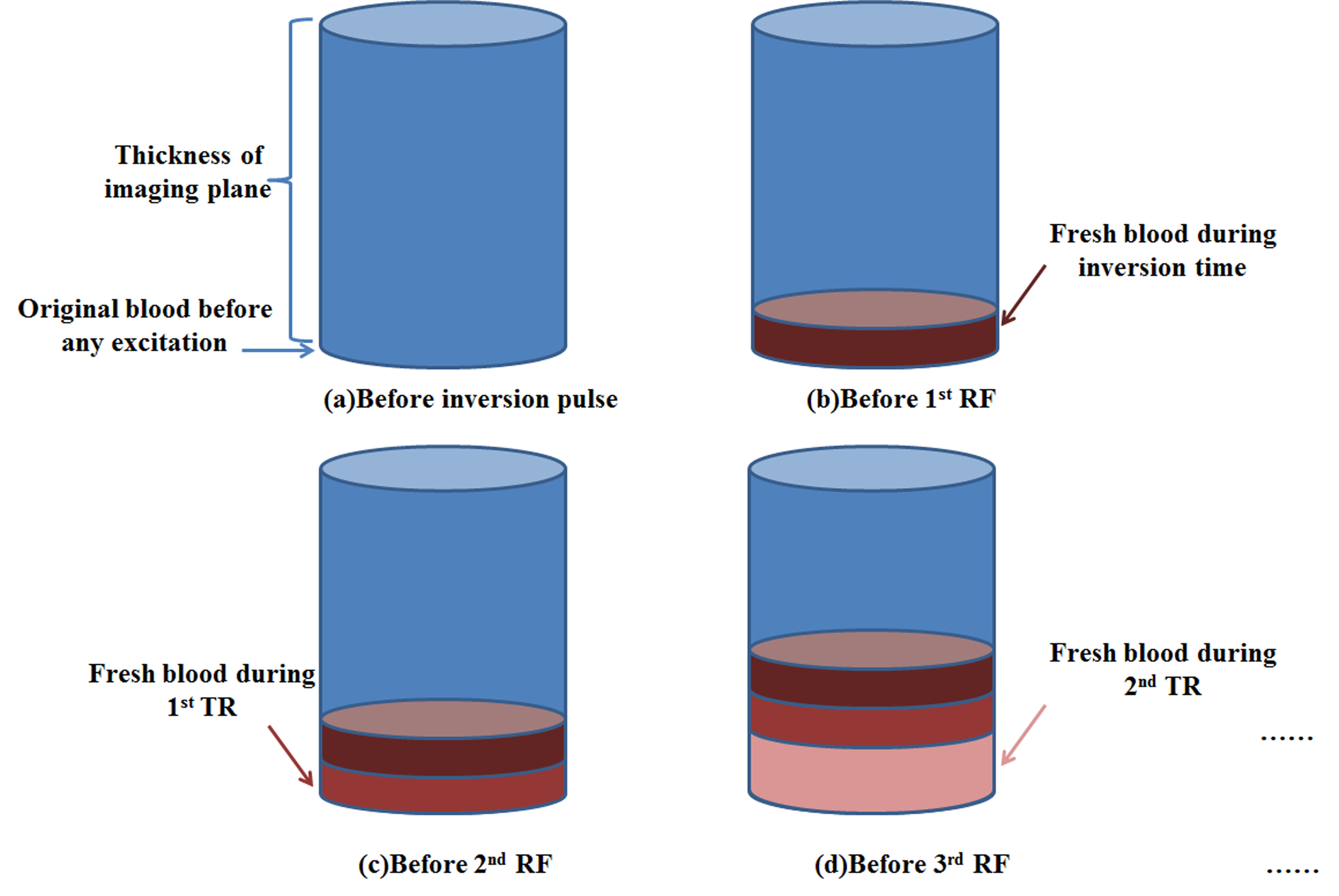
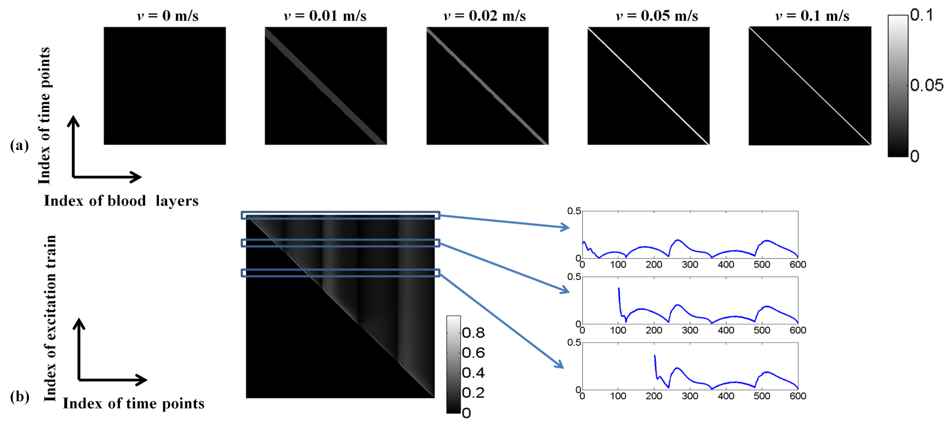
First, a hemodynamic mode was embedded into the extended phase graph (EPG) algorithm ². For simplicity, the velocity of blood flow in vein was assumed as constant during the acquisition and only the blood flow perpendicular to imaging plane (selective slice) was considered. As Figure 1 shows in a simplified brain model for axial imaging, the fresh blood enters the imaging plane from below during each TR and occupies higher position over time, while the dated blood outflows, like a first-in-first-out pipe. So the blood which enters the imaging plane early experiences different excitation train from those that enter later. To simulate this process, a blood-layer ratio matrix $$$ \bf S_{\it v} $$$, calculated with given TRs, slice thickness and velocity v, was used to describe the ratio of the thickness of each blood layer that enters the imaging plane at time t (as Figure 1 shows) to the imaging plane. Matrix $$$ \bf E_{\it T_{\tt1},T_{\tt2}} $$$, calculated by EPG algorithm with given T₁ and T₂, contains signal evolution curves under different excitation trains. Figure 2 shows an example of $$$ \bf S_{\it v} $$$ and $$$ \bf E_{\it T_{\tt1},T_{\tt2}} $$$. In this way, the simulated signal evolution (dictionary entry) $$$ \bf D_{\it v,T_{\tt1},T_{\tt2}} $$$ with introduced velocity dimension could be obtained by:

$$ \bf D_{\it v,T_{\tt1},T_{\tt2}}=diag(\bf S_{\it v}\bf E_{\it T_{\tt1},T_{\tt2}}) $$

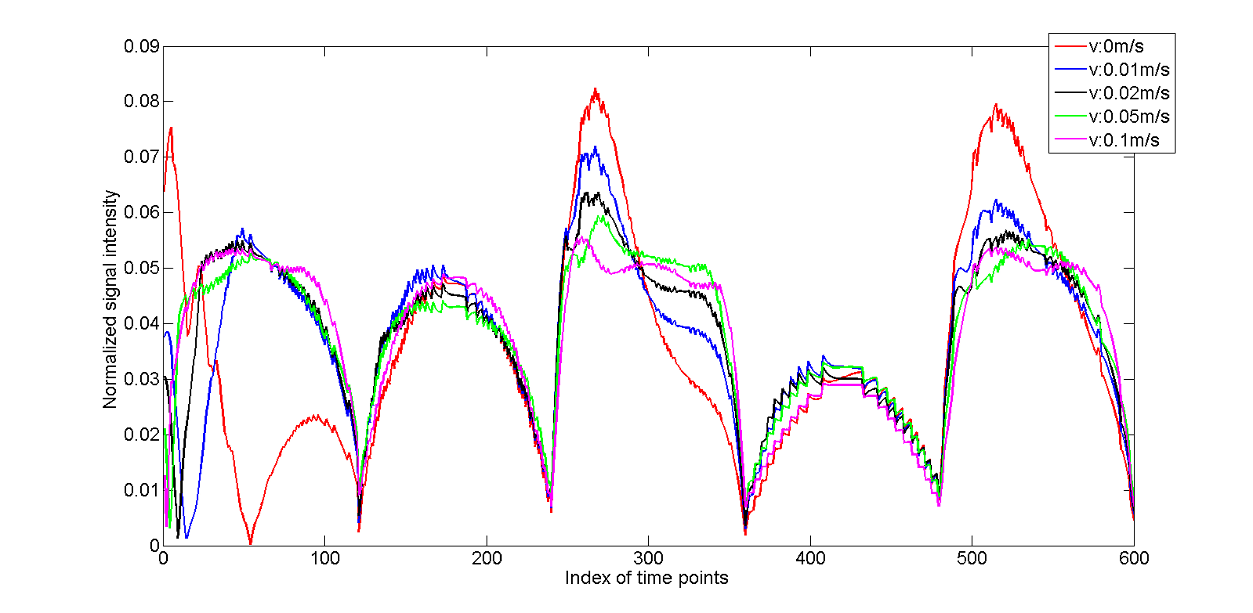
Figure 3 shows $$$ \bf D_{\it v,T_{\tt1},T_{\tt2}} $$$ with varying velocity values (from 0 to 0.1 m/s) and constant T₁/T₂ (1000/100 ms). Significant changes in signal intensity curves demonstrate that the velocity of blood flow implements a strong weighting on the signal evolution. Subsequent processing steps are same with original MRF template matching process.

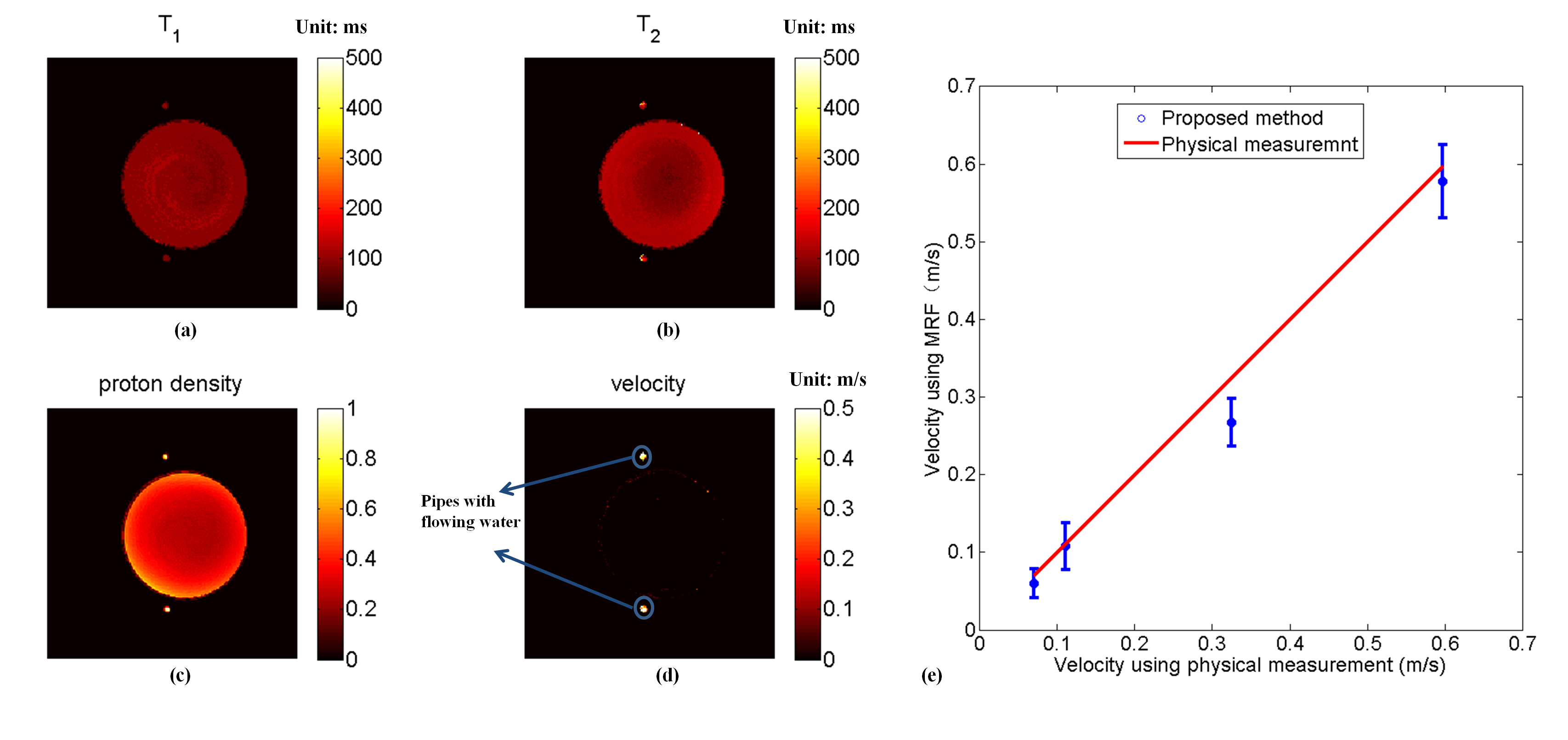
The measurements of a phantom and brain were performed on a Siemens 3T Prisma scanner with a 20 channel head coil. FISP-MRF sequence was used for acquisition ³ with a slice-selective inversion pulse (inversion time = 10 ms). The number of time points used was 600. TRs varied from 9 to 11 ms, and flip angles from 5 to 80 degrees. The thickness of selective slice was 5 mm. The range of T₁ in dictionary was from 20 to 6000 ms, T₂ from 10 to 3000 ms, and velocity from 0 to 1 m/s.

Results and Discussion

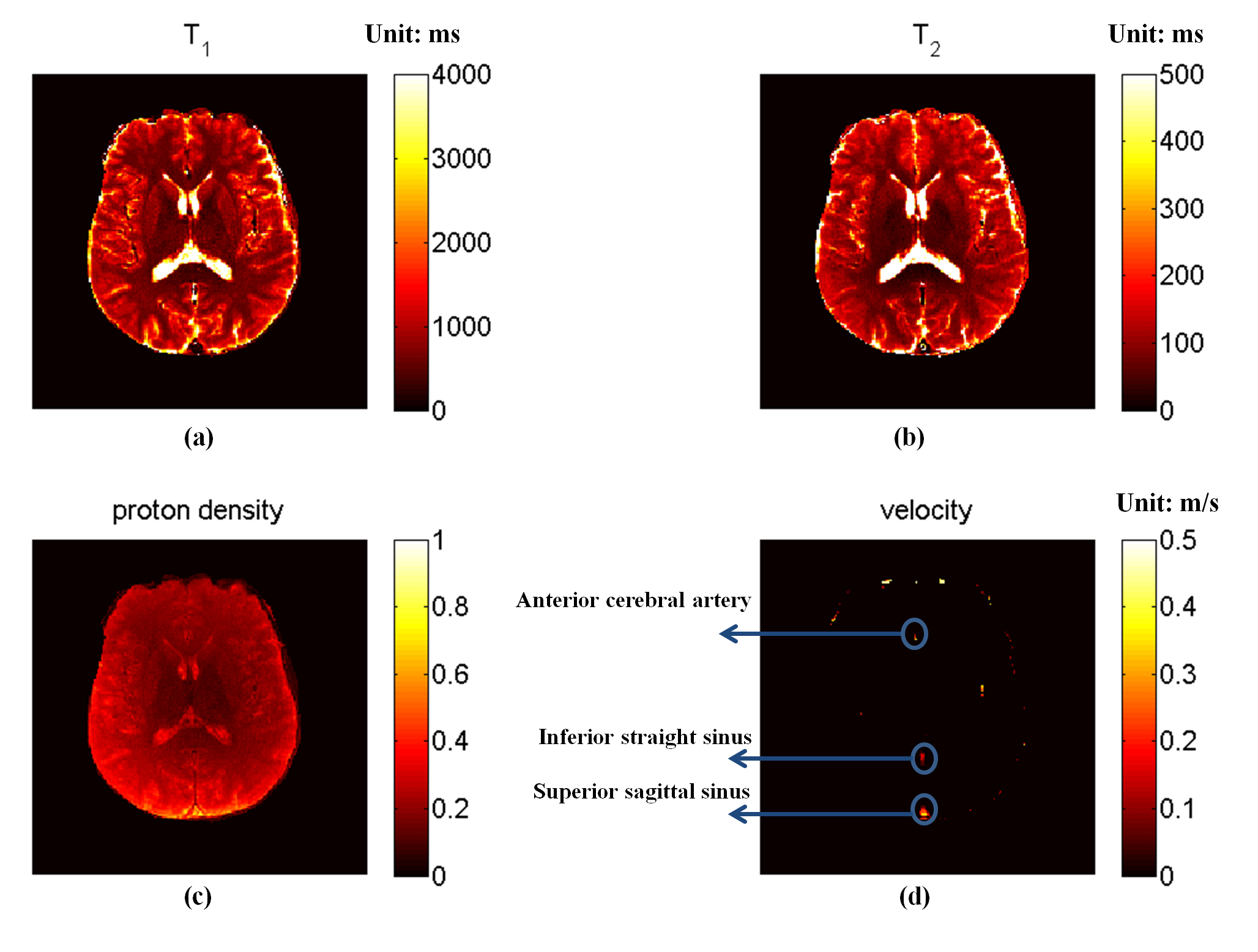
Figure 4 shows the results of the phantom study while Figure 5 shows the obtained T₁, T₂, proton density and velocity maps of a slice within in-vivo brain. Velocity values of blood flow in superior sagittal sinus (0.21±0.04 m/s) is in accordance with reported values (0.23±0.03 m/s) ⁴. However, the velocity of inferior straight sinus is obviously slower than reported values (0.13±0.03 m/s compared with 0.19±0.07 m/s ⁵ ). Since the inferior straight sinus was at an angle across the imaging plane, the obtained velocity values should be the perpendicular components of real velocity, and the obtained velocity appeared slower. To solve this problem, 3D images (or at least adjacent slices) should be acquired, so the directions and angles of veins could be obtained to calculate the real velocity. Besides, the velocity of anterior cerebral arteries had a severe fluctuation (0.27±0.11 m/s), which may be due to the periodical fluctuation of flow velocity during the cardiac circle.

The proposed method builds a dictionary with the introduced velocity measurement and results demonstrate that the proposed method enables velocity mapping without sacrificing quality of the T₁ and T₂ measurements. This is not surprising since the dictionary entries with v=0 are completely the same with original MRF dictionary, and consequently the T₁ and T₂ maps in the areas with v=0 would not change compared with the original MRF.

The velocity value of cerebral veins is an indicator of many diseases like thrombus, stroke, achondroplastic, hypertension, etc ^{6, 7}. However, the hemodynamic model used in this work is simplified. For now only the blood flow perpendicular to imaging plane was considered and the velocity was assumed as constant during acquisition, and therefore the method is mostly applicable to venous blood. To obtain more complicated hemodynamic information, a more sophisticated model must be achieved.

Acknowledgements

References

[1] Ma D, Gulani V, Seiberlich N, Liu K, Sunshine JL, Duerk JL, Griswold MA. Magnetic resonance fingerprinting. Nature 2013;495(7440):187-192.

[2] Weigel M. Extended phase graphs: dephasing, RF pulses, and echoes - pure and simple. J Magn Reson Imaging 2015;41(2):266-295.

[3] Jiang Y, Ma D, Seiberlich N, Gulani V, Griswold MA. MR fingerprinting using fast imaging with steady state precession (FISP) with spiral readout. Magn Reson Med 2015;74(6):1621-1631.

[4] Kuriyama N, Tokuda T, Yamada K, et al. Flow Velocity of the Superior Sagittal Sinus Is Reduced in Patients with Idiopathic Normal Pressure Hydrocephalus[J]. Journal of Neuroimaging, 2011, 21(4): 365-369.

[5] De Boorder M J, Hendrikse J, Der Grond J V, et al. Phase-Contrast Magnetic Resonance Imaging Measurements of Cerebral Autoregulation With a Breath-Hold Challenge A Feasibility Study[J]. Stroke, 2004, 35(6): 1350-1354.

[6] Gideon P, Sorensen P S, Thomsen C, et al. Assessment of CSF dynamics and venous flow in the superior sagittal sinus by MRI in idiopathic intracranial hypertension: a preliminary study.[J]. Neuroradiology, 1994, 36(5): 350-354.

[7] Hirabuki N, Watanabe Y, Mano T, et al. Quantitation of Flow in the Superior Sagittal Sinus Performed with Cine Phase-contrast MR Imaging of Healthy and Achondroplastic Children[J]. American Journal of Neuroradiology, 2000, 21(8): 1497-1501.