0937
Calculation of Large MRF Dictionaries with Low Memory Overhead Using Randomized SVD1Department of Radiology, Case Western Reserve University, Cleveland, OH, United States, 2Department of Biomedical Engineering, Case Western Reserve University, Cleveland, OH, United States
Synopsis
Direct calculation of MRF dictionaries can be prohibitive when high resolution or multi-component chemical exchange effects are taken into account. To address this problem, we propose a new approach based on the randomized SVD (rSVD) to generate a low rank approximation of the large sized dictionary without the need of pre-calculating, storing, or loading the dictionary. This in return saves significant amounts of memory, and speeds up the template matching process of MRF. In addition, when combined with polynomial fitting, one can generate MRF maps with arbitrary high resolution dictionaries.
Purpose
MRF1 matches each voxel signal evolution against a pre-calculated dictionary based on the simulations of signal evolutions with different combinations of parameters of interest, such as $$$T_1,T_2$$$, and off-resonance. The direct calculation of a dictionary, however, could be prohibitive due to memory constraint even for modern computers, especially when a high resolution dictionary is needed or multi-component chemical exchange effects are taken into account2.
We propose a new approach based on the randomized SVD (rSVD)3 to generate a low rank approximation to large sized dictionaries without the need of pre-calculating, storing, or loading the dictionary. This can save significant amounts of memory, and speed up the template matching process of MRF. In addition, when combined with polynomial fitting, one can generate MRF maps with arbitrary high resolution dictionaries.
Methods
Previous studies have shown that MRF dictionaries can be significantly compressed using e.g. the SVD4. Consider a dictionary $$$D\in\mathbb{C}^{t\times{n}}$$$, with $$$t$$$ the number of time frames and $$$n$$$ the number of tissue parameters. Let $$$\Omega\in\mathbb{C}^{n\times{k}}$$$ be a Gaussian matrix drawn from normal distribution with mean 0 and variance 1, where $$$k$$$ is the low rank desired. We embed the tissue property dimension $$$n$$$ into a much lower dimension $$$k$$$ by $$$X=(DD^*)^pD\Omega$$$ with the power iteration index $$$p=0,1,2,\ldots$$$, and perform QR factorization $$$X=QR$$$, where $$$p$$$ depends on the MRF sequence generating the dictionary. Form the matrix $$$Y=Q^*D$$$ and compute its SVD $$$Y=\tilde{U}\Sigma{V}^*$$$. Form the orthonormal matrix $$$U=Q\tilde{U}$$$. We have $$$D\approx U\Sigma{V}^*$$$, where the dimensions of $$$U,\Sigma$$$, and $$$V$$$ are $$$t\times{k},k\times{k}$$$, and $$$n\times{k}$$$ respectively. The template matching for given test signal $$$\boldsymbol{s}$$$ is then computed via $$$\max{D^*\boldsymbol{s}\approx(V\Sigma^*)(U^*\boldsymbol{s})}$$$. Note that in real implementation, $$$D$$$ does not need to be pre-computed and stored. Only one tissue property entry at a time is computed on-the-fly to update the calculation of $$$U,\Sigma$$$ and $$$V$$$, which are much smaller than $$$D$$$, resulting in a significant reduction in the required memory.
We use three types of dictionaries to test the performance of our method: an MRF-FISP5 dictionary, an MRF-bSSFP1 dictionary, and an MRF-X2 dictionary. The MRF-FISP dictionary contains 3,000 time frames and 5,970 different tissue property combinations with $$$T_1$$$ values ranging from 10ms to 2,950ms and $$$T_2$$$ values ranging from 2ms to 500ms ($$$T_2\le{T_1}$$$). The MRF-bSSFP dictionary contains 500 time frames, 500,112 tissue property and off-resonance combinations with $$$T_1$$$ values ranging from 20ms to 5,900ms, $$$T_2$$$ values ranging from 5ms to 2,900ms ($$$T_2\le{T_1}$$$), and off-resonance frequencies ranging from -300Hz to 300Hz. The MRF-X dictionary contains 3,000 time frames and 1,409,232 different combinations of two-component $$$T_1,T_2$$$, volume fraction parameters , and a chemical exchange rate of 0.1s-1.
The brain datasets used for evaluation include three in vivo scans of healthy volunteers. One was obtained on a Siemens Espree 1.5T (Siemens Healthcare, Erlangen, Germany) using the MRF-bSSFP sequence with a matrix size of $$$128\times128$$$ and a field-of-view of 25cm2. The other two were collected on a Siemens Skyra 3T (Siemens Healthcare, Erlangen, Germany) using the MRF-FISP and MRF-X sequences respectively with matrix sizes of $$$256\times256$$$ and $$$192\times192$$$, and field-of-view of 30cm2.
Results
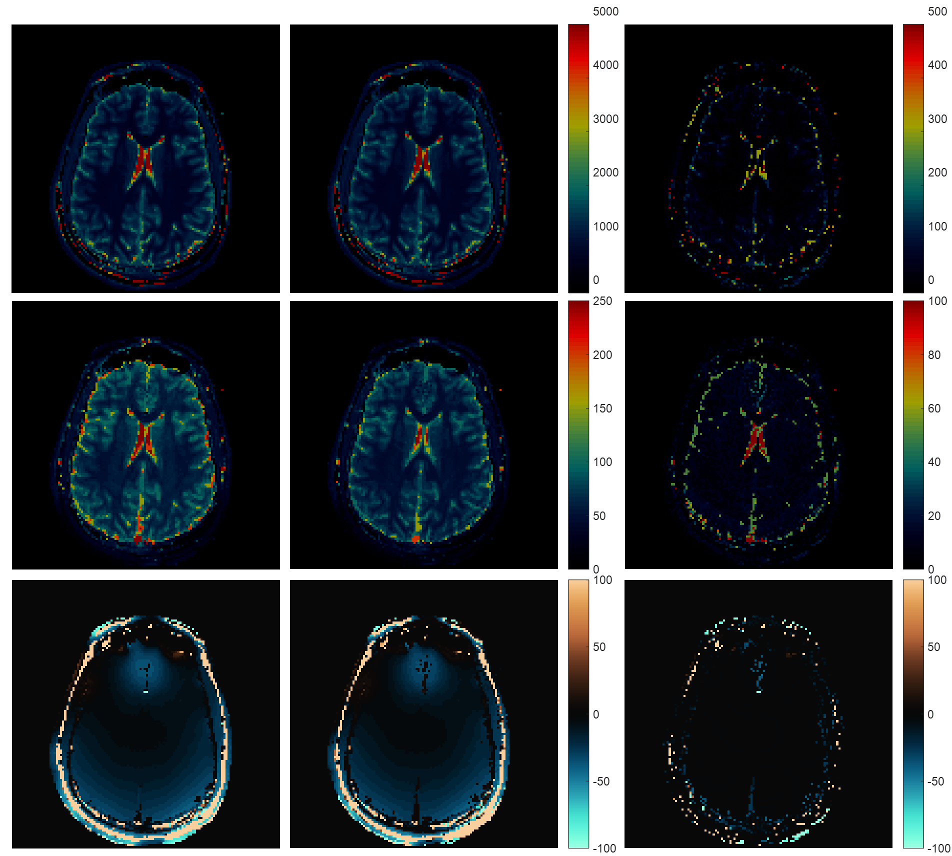
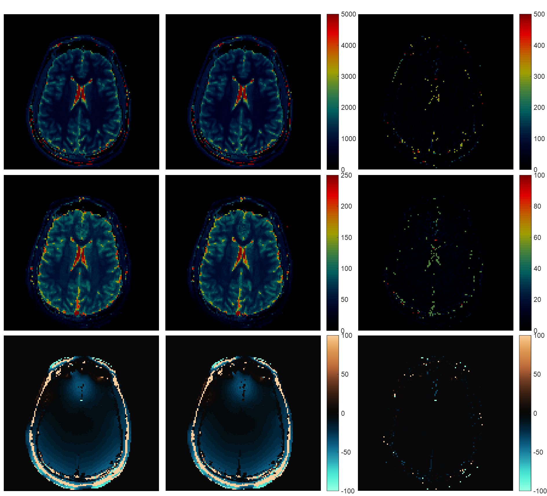
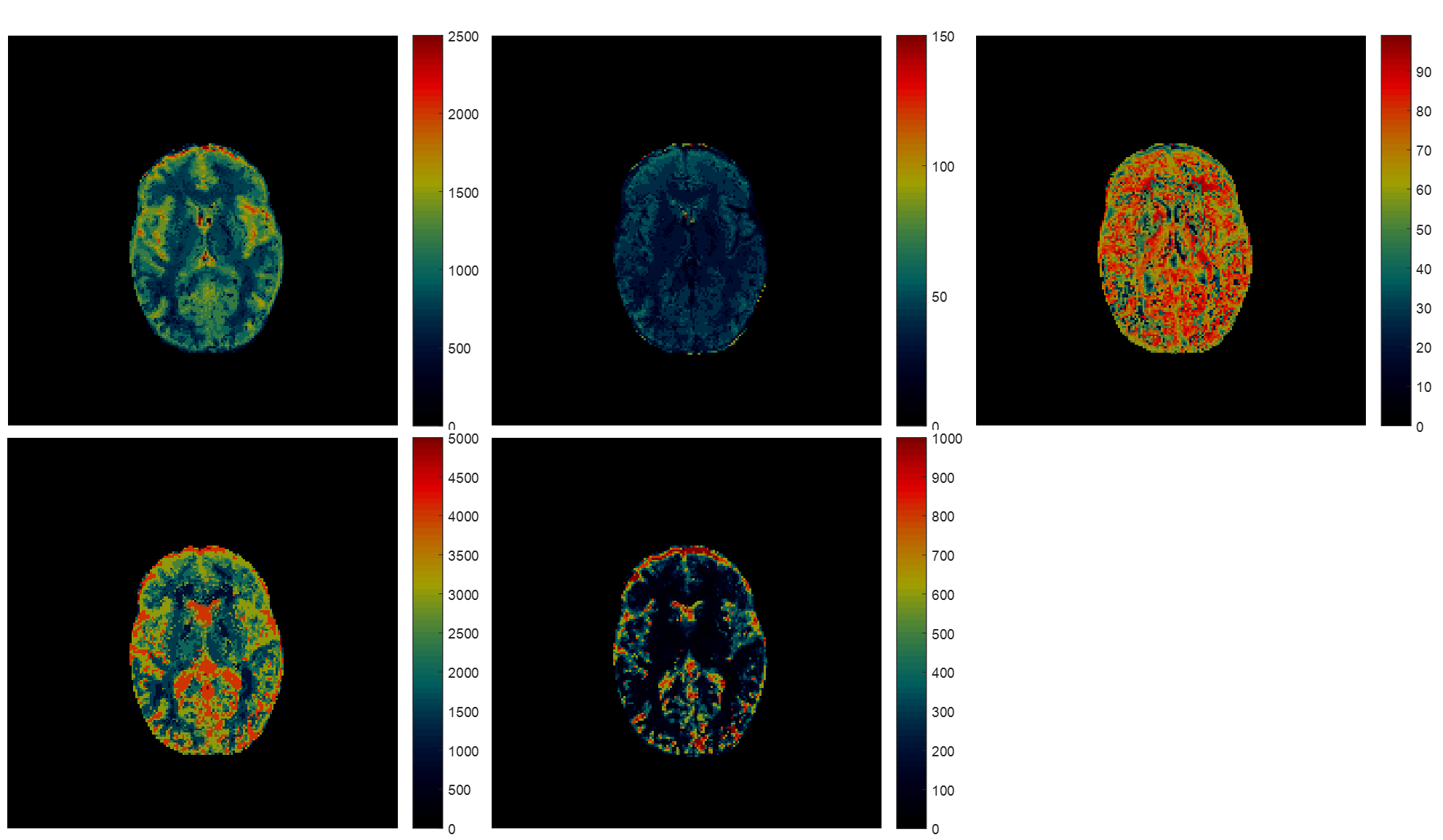
Fig.1 shows the results of applying rSVD to MRF with rank $$$k=30$$$ to the brain dataset obtained from the MRF-FISP acquisition. Fig.2 and Fig.3 demonstrate the results of applying the method with $$$k=100$$$ to the brain data obtained from the MRF-bSSFP acquisition, with power $$$p=0,2$$$ respectively. Fig.4 shows the potential of this approach applied to the very large MRF-X dictionary, where pre-computing, storing, and loading the dictionary is prohibitive.
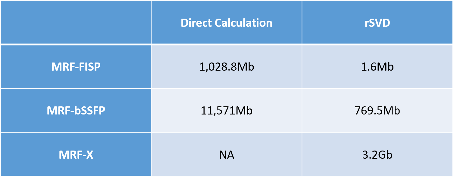
The memory consumption details are shown in Table.1. The memory savings for calculating the MRF-FISP dictionary is almost 1,000 times using our rSVD method against the direct computation. For the MRF-bSSFP calculation using rSVD, the savings is still around 15 times. The direct calculation of the MRF-X dictionary is infeasible on a 64Gb-memory computer, while the memory consumption using rSVD is 3.2Gb.
Discussion and Conclusion
This work proposes a new low rank approximation approach for MRF when calculation of large multidimensional dictionaries is infeasible. Only one tissue property signal evolution at a time is calculated to update the rSVD process, and can be discarded afterwards. This results in significant memory savings for calculating MRF dictionaries. Moreover, when the decay of the singular values is not fast enough, as in MRF-bSSFP, setting the power iteration index properly ($$$p=2$$$ is typically enough) reduces the error significantly. The MRF-X parameter values we show here are not realistic given the fixed chemical exchange rate. However, given the amount of memory savings rSVD achieves, it has great potential in such problems when combined with other methods, such as dictionary fitting.Acknowledgements
The authors would like to acknowledge funding from Siemens Healthcare, grants from NIH 1R01EB016728-01A1, 5R01EB017219-02, and R01HL094557, grants from NSF/CBET 1553441.References
1. D. Ma, V. Gulani, N. Seiberlich, K. Liu, J. L. Sunshine, J. L. Duerk, and M. A. Griswold, Magnetic resonance fingerprinting. Nature 2013, 495:187–192.
2. J. Hamilton, A. Deshmane, M. A. Griswold, and N. Seiberlich, MR Fingerprinting with Chemical Exchange (MRF-X) for In Vivo Multi-Compartment Relaxation and Exchange Rate Mapping, Proc. Intl. Soc. Mag. Reson. Med. 24 (2016), 0431.
3. N. Halko, P. G. Martinsson, and J. A. Tropp, Finding Structure with Randomness: Probabilistic Algorithms for Constructing Approximate Matrix Decompositions, SIAM Review 2011 53:2, 217-288.
4. D. F. McGivney, E. Pierre, D. Ma, Y. Jiang, H. Saybasili, V. Gulani, and M. A. Griswold, SVD Compression for Magnetic Resonance Fingerprinting in the Time Domain. IEEE Transactions on Medical Imaging, vol. 33, no. 12, pp. 2311-2322, Dec. 2014.
5. Y. Jiang, D. Ma, N. Seiberlich, V. Gulani, and M. A. Griswold, MR fingerprinting using fast imaging with steady state precession (FISP) with spiral readout. Magn. Reson. Med. 2015, 74: 1621–1631.
Figures