Synopsis

We reconsider balanced gradient-echo (GRE) sequence for MR fingerprinting and design an excitation scheme which is very robust to off-resonance. The corresponding data can be accurately reconstructed by standard least-squares fitting methods, a novelty for MRF. Construction of the pre-computed dictionary and exhaustive search are thus no longer needed.

Purpose and Introduction

MR fingerprinting (MRF)^[1] reconstructs $$$T_1,T_2$$$ and proton density ($$$\rho$$$) from series of highly undersampled images by means of an exhaustive search over a pre-computed dictionary. The dictionary-match is troublesome when applied to balanced GRE sequences due to their sensitivity to off-resonances ($$$\Delta_{\omega}$$$)^[2]. Therefore, the MRF community is focusing on spoiled sequences, which are much less dependent on off-resonance^[3].

Balanced sequences do have important advantages over spoiled sequences, such as higher SNR and robustness to motion. Here, we reconsider balanced GRE sequence for MRF and design an excitation scheme which is very robust to off-resonance. The corresponding data can be accurately reconstructed by standard least-squares fitting methods, a novelty for MRF. Construction of the pre-computed dictionary and exhaustive search are thus no longer needed.

Theory

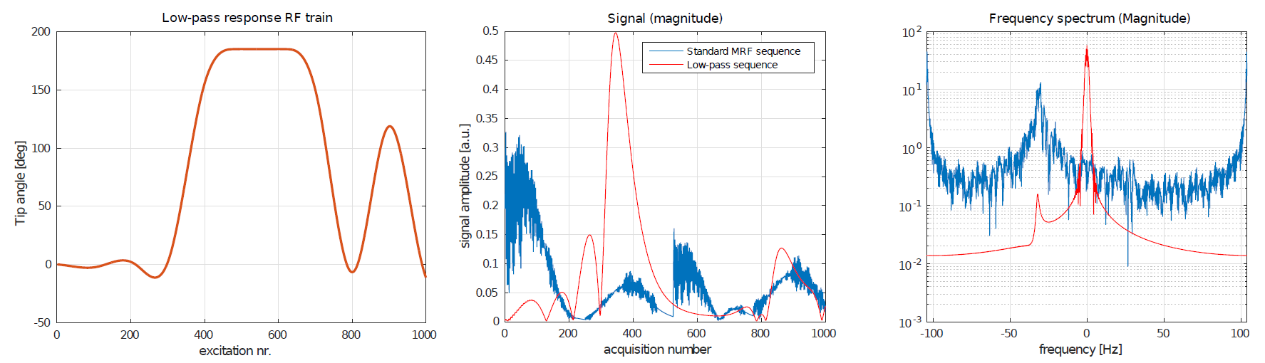
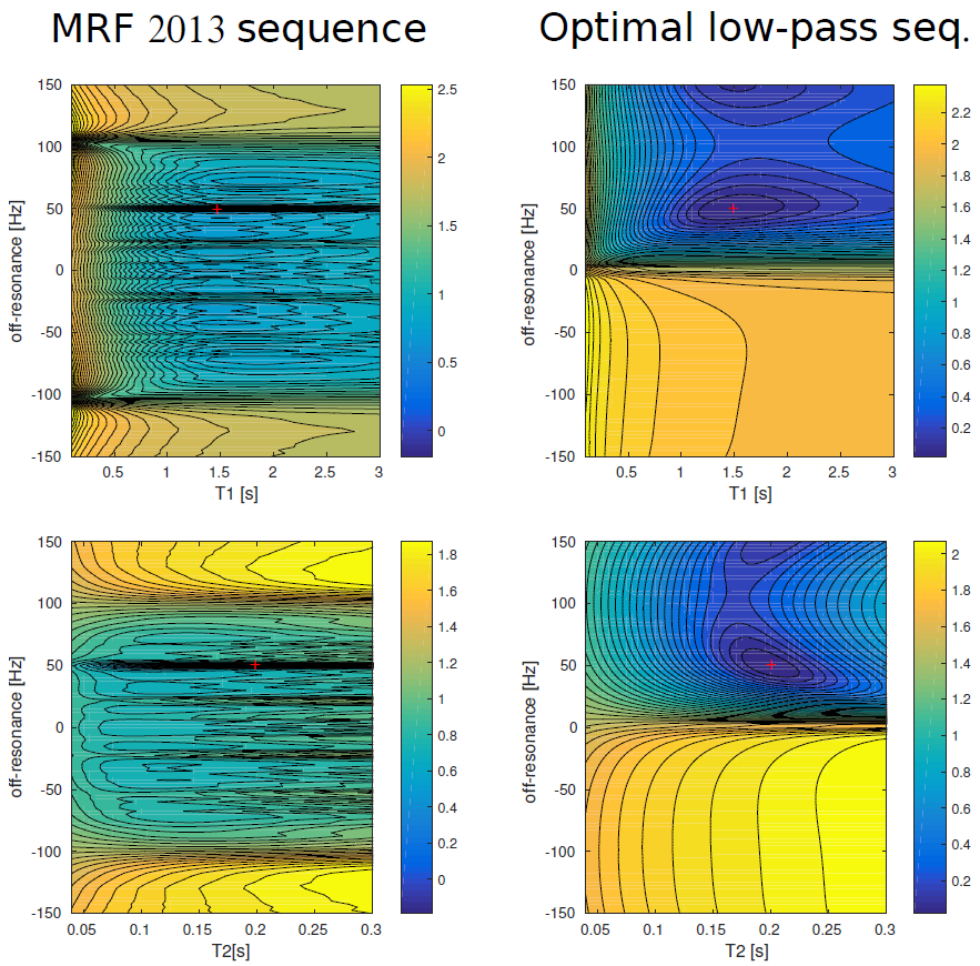
MRF signals show large high-frequency components originating from $$$k$$$-space undersampling but also from the inherently high-frequency response of the MRF sequence as shown in Fig.1. Therefore, nonlinear least-squares fitting algorithms can not separate the true signal component from the perturbations and local minima (thus wrong parameters) are attained. Fig.2 shows the irregular minimization landscapes of a standard MRF sequence, characterized by many suboptimal solutions.

The rationale for our method is that the undersampling artifacts should come in a high-frequency band while the true signal evolution, which is connected to $$$T_1$$$ and $$$T_2$$$ quantification, in low- frequency band. A sequence with such response allows for better separation between the true signal evolution and the aliasing artifacts. For these type of sequences, the Bloch-based least-squares fitting will function as a low-pass filter and we call them low-pass sequences.

In addition to the smooth response, the low-pass sequence should also be highly sensitive to the parameters of interest i.e. $$$\rho,T_1,T_2$$$. The sensitivity of an estimation problem can be directly quantified by the diagonal entries of the covariance matrix of the model, which are an estimate for the standard deviation, $$$\sigma$$$, of the corresponding parameter. Obviously, $$$\sigma$$$ should be as small as possible.

Methods

A low-pass sequence is characterized by a smooth tip-angle train with starting value $$$\theta(0)=0$$$ (see Fig.1).

To enhance the sensitivity to the parameters while ensuring a low-frequency response we solve:

$$\begin{array}{rl} \text{Minimize with respect to }\theta(t):&\max\left\{\frac{\sigma(T_1^n)}{T_1^n},\frac{\sigma(T_2^n)}{T_2^n},\frac{\sigma(\rho^n)}{\rho^n}\quad\forall n\right\}\\ \text{such that:}&\theta(0)=0\\ &\frac{\text{d}\theta}{\text{d}t}\leq\delta\quad\text{(low-pass constraint)}\\ &\theta(t)\leq180^{\text{o}}\quad\text{for}\quad t\in[0,T]\end{array}$$

where $$$\theta(t)$$$ denotes the tip-angle and the standard deviation $$$\sigma$$$ is calculated from the covariance of the Bloch equation model. $$$n$$$ runs over a test-set of 25 different values of $$$(T_1,T_2,|B_1^+|,\Delta_{\omega})$$$ which are randomly drawn in the range:

$$ \begin{array}{rcl} T_1&\in&[250,3000]\text{ms}\\T_2&\in &[50,250]\text{ms}\\|B_1^+|&\in&[0.9,1.1]\text{a.u.}\\ \Delta_{\omega}&\in &[-150,150]\text{Hz}. \end{array}$$

$$$\theta$$$ is parametrized by 10 cubic-spline functions, ensuring a smooth tip-angle variation. $$$(T_E,T_R)=(2.4,4.8)$$$ms, 1000 excitations.

For the reconstructions, we first consider a $$$128\times128$$$ digital brain phantom[4] with typical 1.5T off-resonance and RF transmit field variation $$$(\Delta_{\omega}\in[-150,+150]$$$a.u., $$$B_1^+\in[0.9,1.0]$$$a.u.). The high-frequency undersampling artifacts are simulated as Gaussian random perturbations such that

$$ \frac{\sqrt{\sum_n|\text{true signal}_n|^2}}{\sqrt{\sum_n|\text{artifacts}_n|^2}}=3.$$

The corrupted brain images are reconstructed in Matlab by means of:

1) a standard MRF dictionary-search

2) the proposed dictionary-free approach with a quasi-Newton algorithm for nonlinear least-squares.

In addition to the numerical experiments, experimental data was acquired with the original MRF sequence^[1] and the optimized low-pass sequence on a 1.5T scanner (Philips-Ingenia) using a 13-channel coil.

A golden-angle radial-trajectory^[5] was used with resolution=2x2mm$$$^2$$$, slice-thickness=10 mm, FOV=256x256mm$$$^2$$$ and 20 spokes per time-point (10-fold undersampling).

Results

The optimized low-pass sequence is shown in Fig.1-left and its optimization landscapes in Fig.2. Note the smooth response and highly regular landscapes of the low-pass sequence.

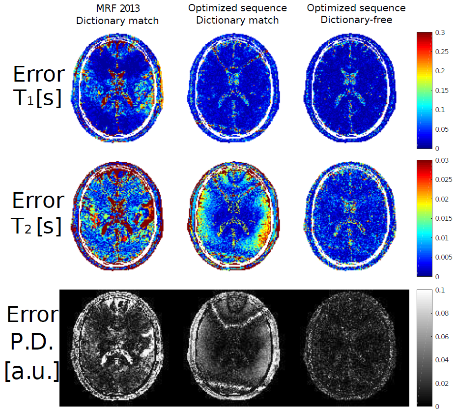
The dictionary-match and proposed least-squares reconstruction of the low-pass sequence along with the dictionary-match from the original MRF sequence are shown in Fig.3. The least-squares approach outperforms the dictionary match in terms of precision for the low-pass sequence. See also the difference maps (Fig.4).

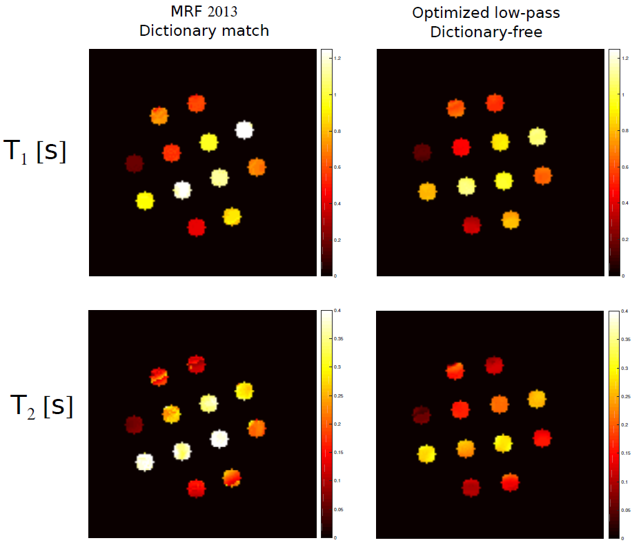
The experimental reconstructions (Fig.5) show that the optimized low-pass scheme is able to reconstruct $$$(T_1,T_2)$$$ over a large dynamic range especially towards large $$$(T_1,T_2)$$$ values. The maps also exhibit lower intra-tube variation than the original MRF flip-angle scheme.

Discussion and conclusions

We reconsider balanced GRE sequences for MRF. We cast the reconstruction as a nonlinear least-squares fitting and we quantify the precision of the reconstruction a priori from statistical analysis. No parameter reconstruction is needed during the sequence design step since the sensitivity of the sequence is directly derived from the flip-angle train.

Based upon this information, we design a balanced sequence with separable frequency bands for true signal and aliasing artifacts. The low-pass sequence exhibits a smooth optimization landscape with very few local minima and is very robust to off-resonance facilitating a dictionary-free reconstruction which returns better results than the standard MRF.

Acknowledgements

The first author is grateful to Dr. Chris Stolk, Dr. Tristan van Leeuwen and Dr. Martijn Cloos for the fruitful discussions.

This presented research was partially funded by the Dutch Technology Foundation (STW) grant 14125.

References

[1] Ma D, Gulani V, Seiberlich N, Liu K, Sunshine JL, Duerk JL, Griswold MA. Magnetic resonance fingerprinting. Nature. 2013 Mar 14;495(7440):187-92.

[2] Doneva M, Amthor T, Koken P, Keupp J, Boernert P. Accuracy Analysis for MR Fingerprinting. In proceedings of the 23rd annual meeting of the International Society for Magnetic Resonance in Medicine. Toronto, Canada. 2015. pag. 3395.

[3] Jiang Y, Ma D, Seiberlich N, Gulani V, Griswold MA. MR fingerprinting using fast imaging with steady state precession (FISP) with spiral readout. Magnetic resonance in medicine. 2015 Dec 1;74(6):1621-31.

[4] Aubert-Broche B, Evans AC, Collins L. A new improved version of the realistic digital brain phantom. NeuroImage. 2006 Aug 1;32(1):138-45.

[5] Cloos MA, Knoll F, Zhao T, Block KT, Bruno M, Wiggins GC, Sodickson DK. Multiparametric imaging with heterogeneous radiofrequency fields. Nature Communications. 2016 Aug 16;7.