0861
Clinical Translation of Tumor Acidosis Measurements with AcidoCEST MRI1Biomedical Engineering, University of Arizona, Tucson, AZ, United States, 2Medical Imaging, University of Arizona, Tucson, AZ, United States, 3University of Arizona Cancer Center, University of Arizona, Tucson, AZ, United States, 4Medicine, University of Arizona, Tucson, AZ, United States
Synopsis
We optimized acidoCEST MRI, a method that measures extracellular pH (pHe), and translated this method for clinical imaging. We fit CEST spectra with the Bloch equations modified to include the direct estimation of pH, and generated parametric maps of tumor pHe in the SKOV3 tumor model, a patient with high grade invasive ductal breast carcinoma, and a patient with metastatic ovarian cancer. AcidoCEST MRI successfully measured a pH 6.58 in a tumor of the patient with metastatic ovarian cancer. The primary breast tumor failed to accumulate sufficient agent to generate pHe measurements.
Purpose
The extracellular pH (pHe) has been measured in tumor models of human cancers with chemical exchange saturation transfer (CEST) MRI, using a method known as “acidoCEST MRI”.1 We aimed to optimize the acidoCEST MRI acquisition protocol for clinical translation by improving our analysis methods to avoid overfitting noisy CEST spectra, especially when CEST signal amplitudes are low.Methods
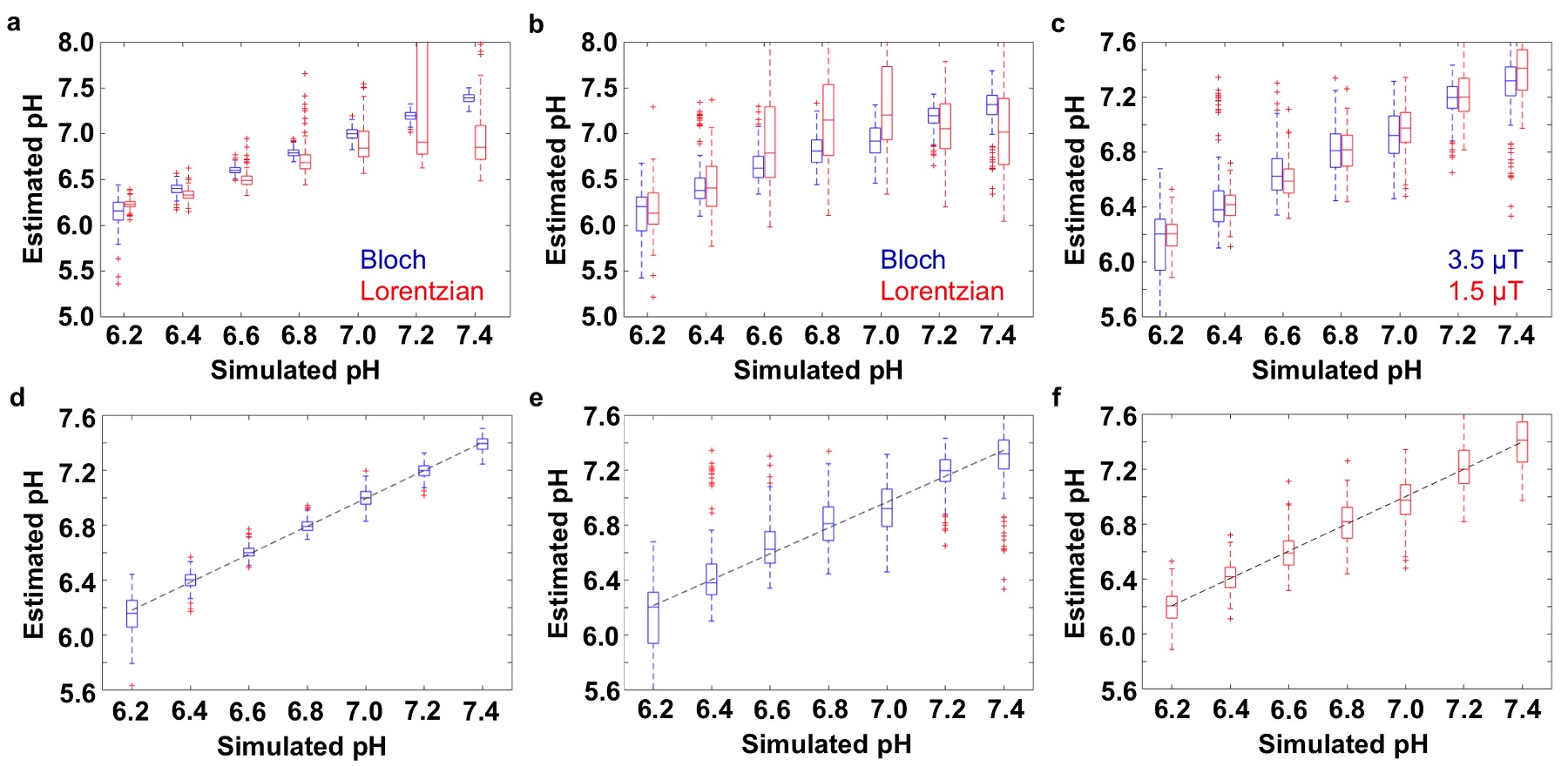
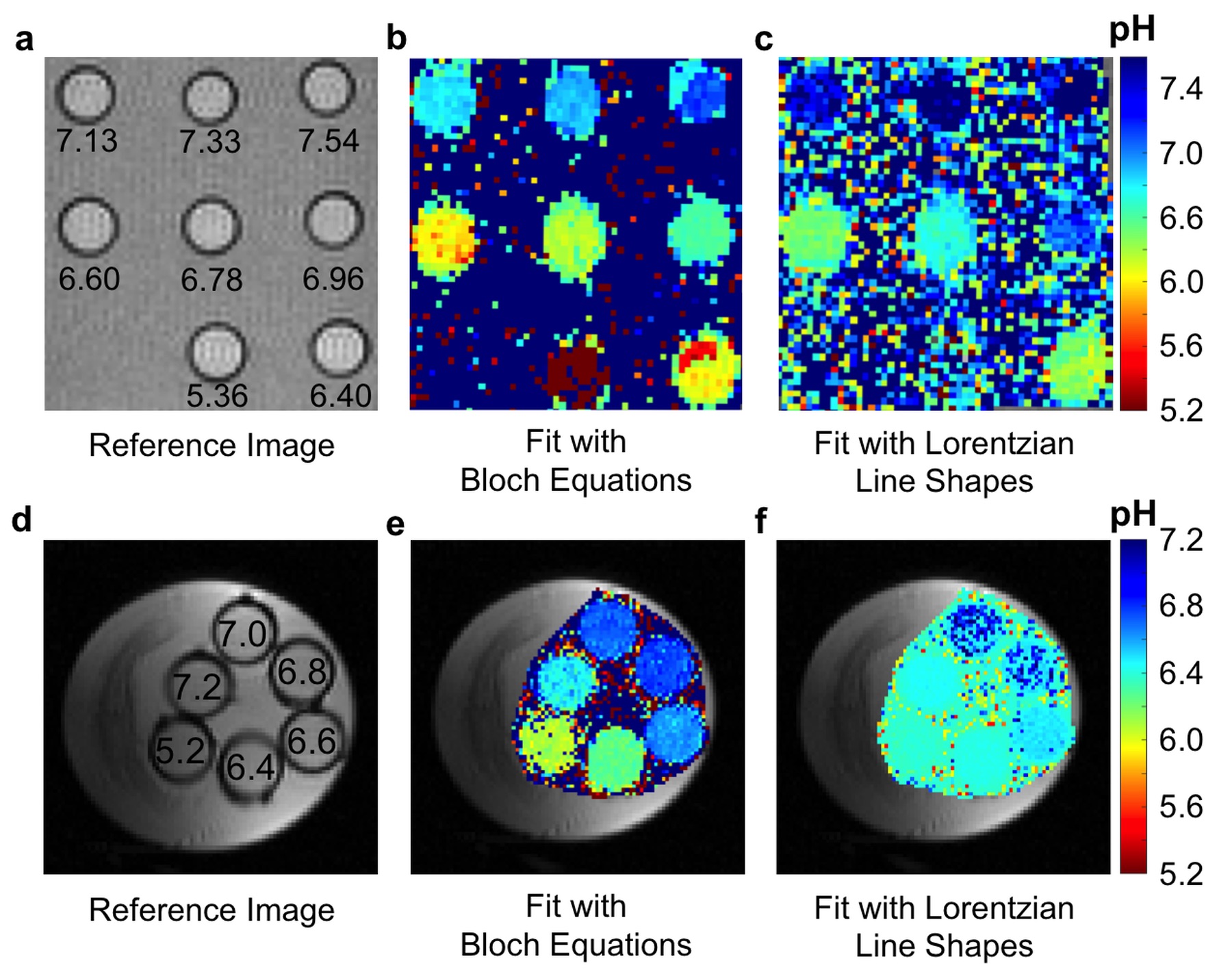
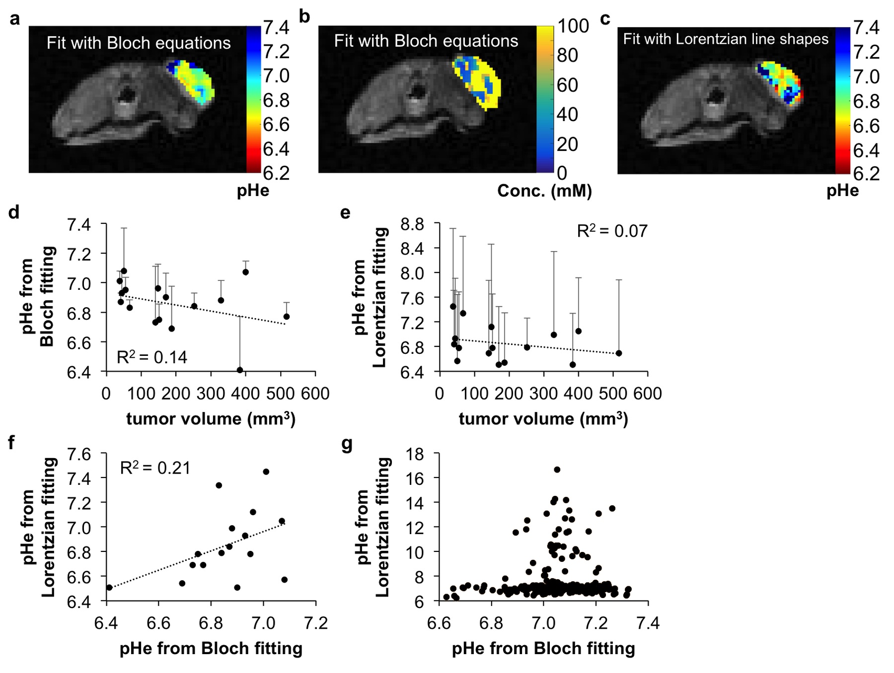
Solutions of 78 mM iopamidol at pH 5.82-7.67 were scanned with an ultrafast CEST MRI method using a 600 MHz NMR spectrometer at 37.0 ± 0.5 °C.2 The uncatalyzed and base-catalyzed exchange rates were determined for each exchanging pool of iopamidol. This analysis allowed us to incorporate the pH into the Bloch equations as a fitting parameter. CEST spectra ranging between pH 6.2-7.4 were simulated with Gaussian noise using the experimentally determined exchange rates of iopamidol.3 The Bloch equations and Lorentzian line shapes were fit to the simulated CEST spectra to estimate the pH value to evaluate each fitting method.3,4 Phantoms of 10 mM iopamidol at pH 5.36-7.54 were scanned with acidoCEST MRI using a 7T Bruker Biospec MRI scanner. Phantoms of 50 mM of iopamidol at pH 5.21-7.22 were scanned with a 3T Siemens Skyra MRI scanner. Ten female mice with a flank tumor of SKOV3 human ovarian cancer were scanned at 7T with a 2 sec saturation pulse at 3.5 mT power. Four pre-injection scans were followed by injection of 3.7 mgI/g iopamidol and infusion of iopamidol at 400 μl/hr, followed by six post-injection acidoCEST MRI scans. The total scan time was 37:50 min.
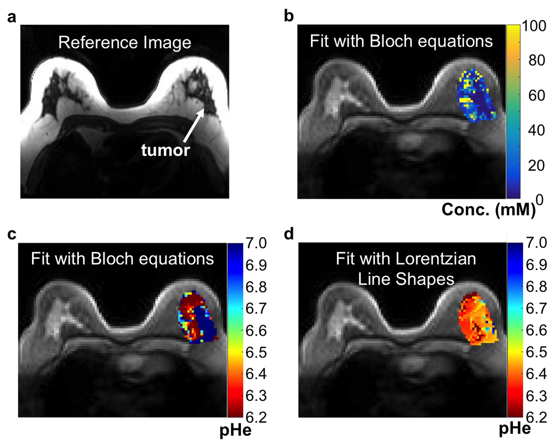
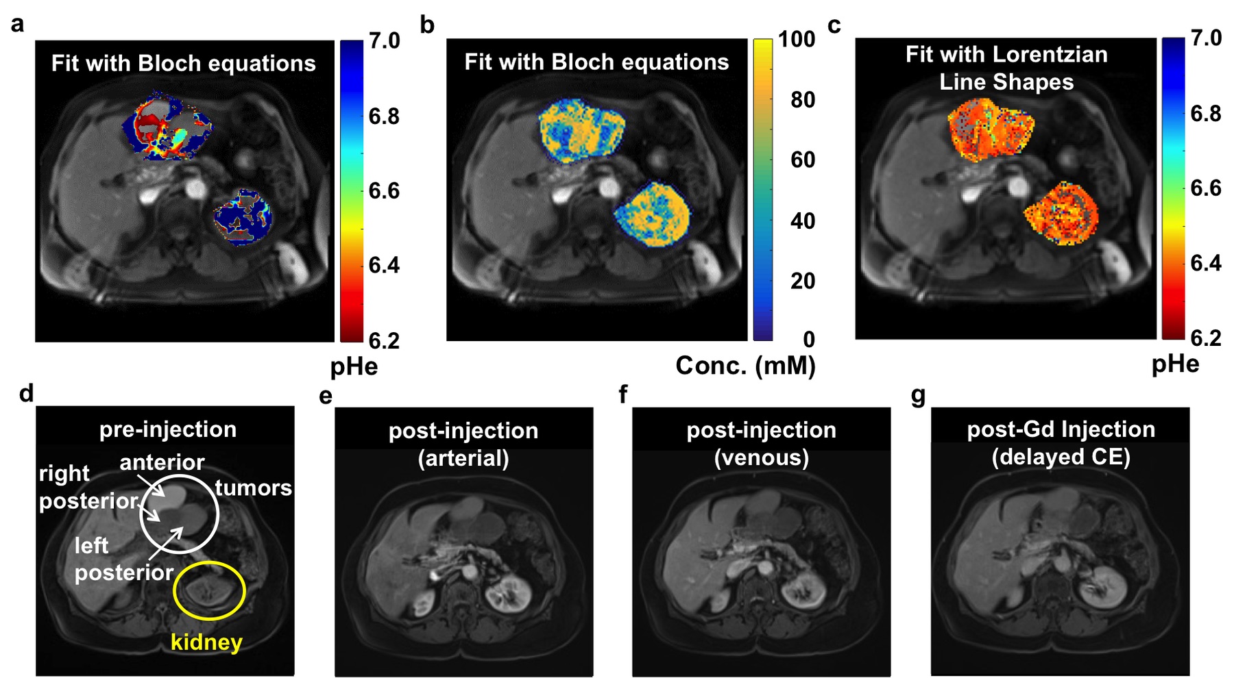
Metastatic peritoneal implants in a patient with high grade serous ovarian carcinoma were scanned with acidoCEST MRI using a 2.0 sec saturation period at 1.5 mT power, and with a turboFLASH acquisition. After 10 pre-injection scans, 60 mL of 370 mgI/mL was injected i.v. over 1 min followed by infusion of another 60 mL at 0.2 ml/s for 5 min, followed by 15 post-injection scans for a total scan time of 23:45 min. A patient was also scanned who presented with a grade I invasive ductal breast carcinoma using the same clinical acidoCEST MRI protocol. For in vivo acidoCEST MRI, the average, spatially smoothed post-injection image was subtracted from the average, spatially smoothed pre-injection image. CEST spectra were constructed for each pixel, and analyzed by fitting CEST spectra with Bloch equations and Lorentzian line shapes.
Results
Simulations showed that Bloch fitting generated more accurate and more precise pH values than Lorentzian fitting at 7T and 3T magnetic field strengths, especially at higher pH values. The precision of pH estimates at 7T was more precise than pH estimates at 3T. Bloch fitting produced more accurate pH estimates with a 1.5 µT saturation power than 3.5 µT at 3T due to better peak separation with a lower saturation pulse power at a lower field strength. Bloch fitting produced reliable pH maps of the SKOV3 model that ranged from pH 6.4 to 7.4 and with a concentration of 5 to 100 mM in the flank tumor. Lorentzian fitting methods were sensitive to noise, and caused overfitting of the CEST spectrum that generated unreasonable values below pH 6.4 and above pH 7.4. The high grade invasive ductal breast carcinoma produced unreliable pHe measurements with Bloch and Lorentzian fitting, which was attributed to low uptake of the agent. Metastatic peritoneal implants in the patient with high grade serous ovarian carcinoma showed 56-84 mM uptake of the agent, allowing for reliable pHe measurements with Bloch fitting. The average pHe value of this right posterior tumor was 6.79 units, and the standard deviation of 0.21 units. The kidney of this patient showed an average pHe of 6.73 units with a standard deviation of 0.24 units. The average concentrations of the agent was 80 mM in the outer cortex and 69 mM in the inner medulla. Lorentzian fitting showed pHe measurements of approximately 6.4 throughout the tumors and kidney, demonstrating poor estimations.Discussion
This study has established the clinical translation of acidoCEST MRI from imaging of a flank tumor murine model to the successful clinical imaging of a patient with metastatic ovarian cancer. The pHe measurements estimated with Bloch fitting compared to Lorentzian fitting were more accurate and precise in simulations, chemical solutions, a flank tumor model, and a patient. pHe measurements could only be made in tissues with high uptake of the agent, which agreed with a previous report.5Acknowledgements
No acknowledgement found.References
1. Chen LQ, et al. Magn Reson Med 2013;72:1408-1417.
2. Dopfert J, et al. J Magn Reson 2014;243:47-53.
3. Woessner DE, et al. Magn Reson Med 2005;53:790-799.
4. Sheth VR, et al. Contrast Media Mol Imaging 2012;1:26-34.
5. Muller-Lutz A, et al. Magn Reson Mater Phy 2014;27:477-485.
Figures