Synopsis

Dynamic contrast enhanced MRI can be used to obtain single-kidney GFR estimates but tradeoffs between spatial and temporal resolution lead to errors. We propose a novel reconstruction technique where AIFs are generated from images reconstructed with high temporal resolution while renal parenchyma signal is extracted from images reconstructed over a larger temporal window to generate images with high spatial resolution and improved image quality. We demonstrate the clinical validity of the method by estimating the GFR using our proposed method and compare it with serum creatinine based eGFR estimate.

Introduction:

Method:

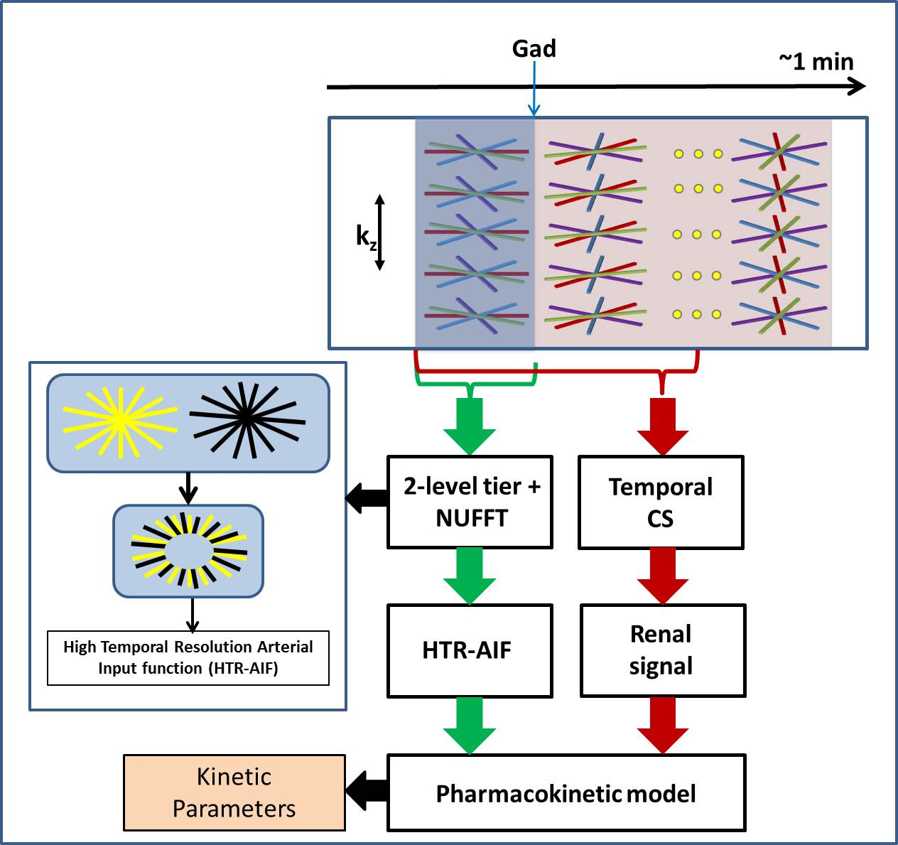
Accurate AIF estimation: The generation of AIF with 1-sec TRES requires images reconstructed from 7 radial views, which have severe streaking artifacts and noise. Furthermore, pre-contrast images suffer from poor SNR, severely compromising the AIF baseline and, hence, GFR accuracy. We used a 2 level tiering reconstruction [3], where central and peripheral k-space spanned 1-sec and 2-sec respectively to generate 1-sec TRES AIF curves (Fig 1 inset). To minimize fluctuations in pre-contrast images where the signal is flat, a 4-sec temporal window was used. A realistic digital phantom synthesized from an in vivo data set [1, 2] and fused AIF curve was used for validation.

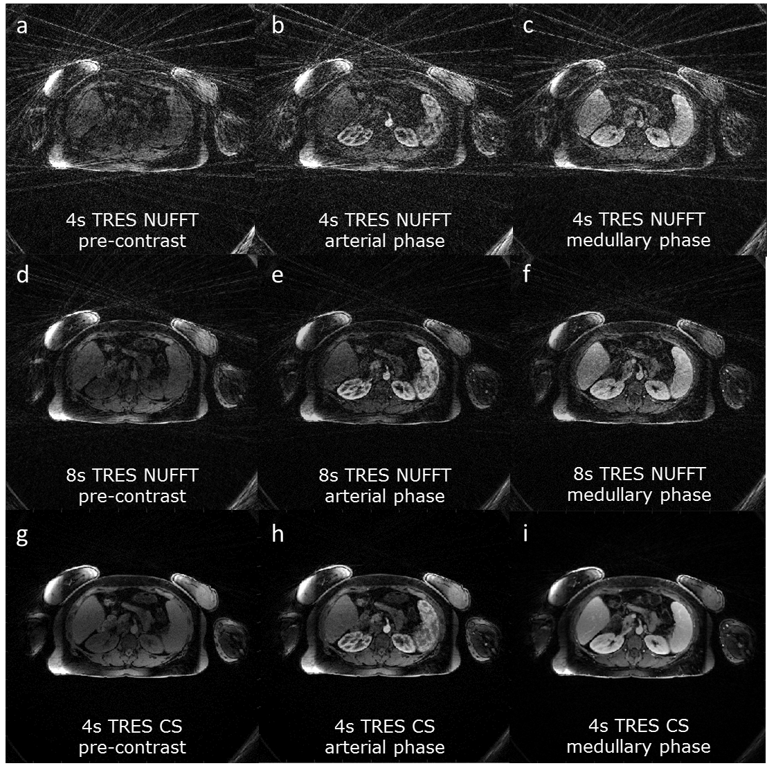
Dynamic renal MRI: To generate diagnostic quality dynamic images, a lower temporal resolution (4-sec) was used along with compressed sensing (CS) to minimize streaking artifacts and residual noise [4]. A Total Variation (TV) sparsity constraint applied across the temporal dimension as shown by following equation.$${d={(}{\arg\min_{d}\ }\|{F.C.d-m}\|}^2_{2}+\lambda\|S.d\|_{1}{)}$$ AIF images used a non-uniform Fast Fourier Transform (NUFFT) to minimize temporal blurring that could result from CS regularization. For image quality comparisons, 4-sec and 8-sec TRES NUFFT images were used.

GFR estimation: A semi-automated segmentation of aortic and parenchymal ROIs was performed. GFR and v_b estimates were computed using a Toft’s 2-compartment model [5]. A paired t-test was used to determine statistical significant to determine if there was a statistically significant difference between MRI based GFR and serum creatinine based eGFR estimates.

Imaging was performed on a 3T MRI scanner (Skyra, Siemens Healthcare, Malvern, PA) using a 3D radial golden angle stack-of-stars spoiled gradient echo sequence on 15 patients referred for lumbar spine or abdominal imaging, after informed consent. Acquisition parameters: TR = 3.52 ms; TE = 1.5 ms; FOV = 38 cm; flip = 10°; acquisition matrix=288x288x44; 3-6 mm slice thickness for whole abdomen coverage. Free breathing 3D radial data were acquired continuously but only 90-sec of data following injection of Gadolinium contrast was used for analysis.

Result:

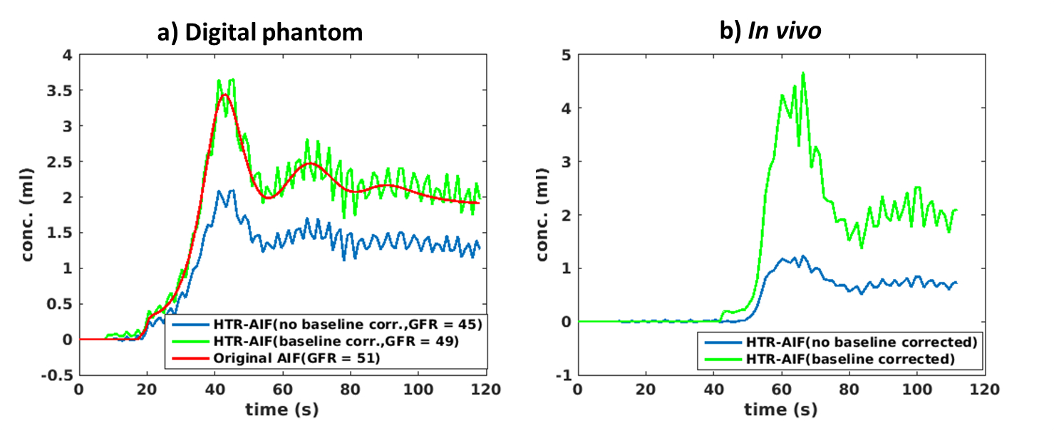
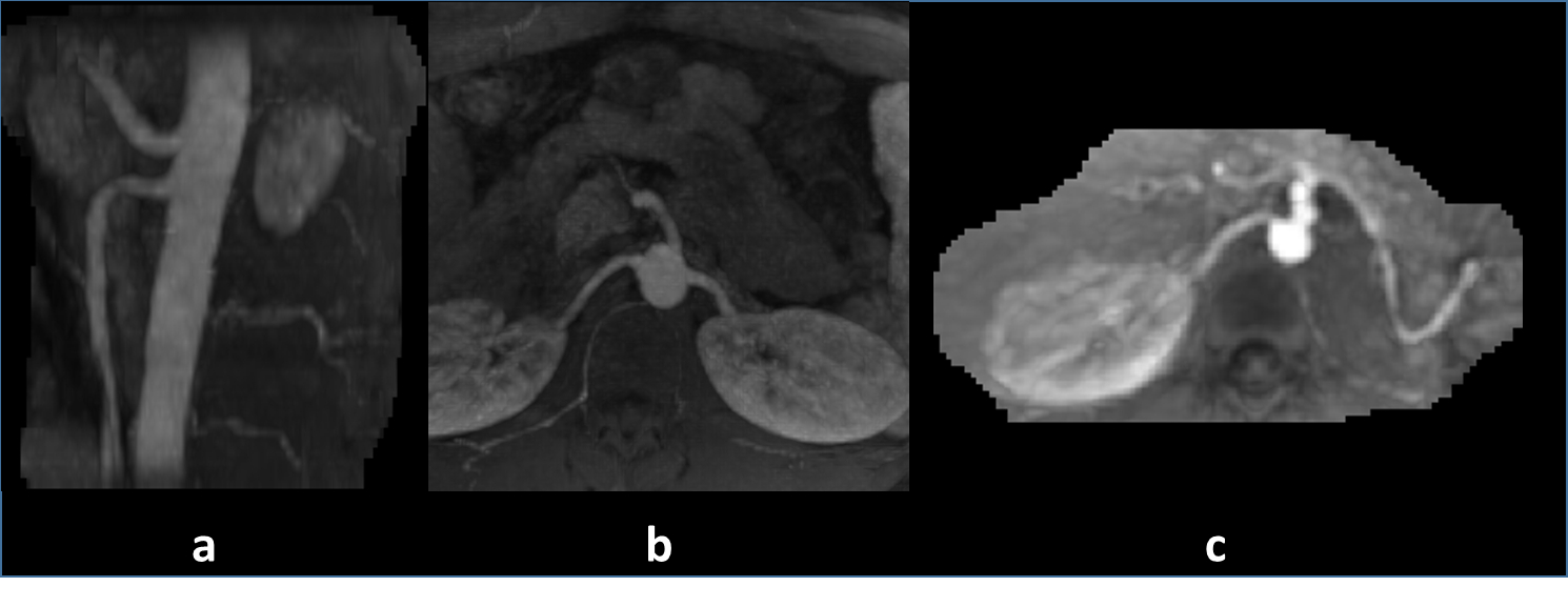
Figure 2 (left) compares 1-sec HTR-AIF curves with (blue) and without (green) 2 level tiering and baseline correction with the true AIF on a digital phantom (red). It can be seen that 2 level tiering and baseline correction significantly improves the AIF and GFR accuracy. Fig. 2 (right) shows the same effect on an in vivo data set, again significantly changing the AIF and GFR values. Figure 3 shows pre-contrast, arterial, and medullary phases from an in vivo data set, reconstructed using 4-sec and 8-sec temporal resolution NUFFT (top and middle rows) compared to 4-sec temporal resolution CS (bottom row). Better image quality (minimal noise/ streaking) can clearly be seen in the CS reconstruction compared to the NUFFT reconstructions. The diagnostic utility of the 4-sec CS images are further illustrated in Figure 4 which shows thin slab MIPs in a patient with no known disease (Fig. 4(a)(b)) and a patient (c) whose left kidney was removed. The visualization of small branching vessels and the absence of venous signal attest to the high spatio-temporal resolution achieved by our technique.

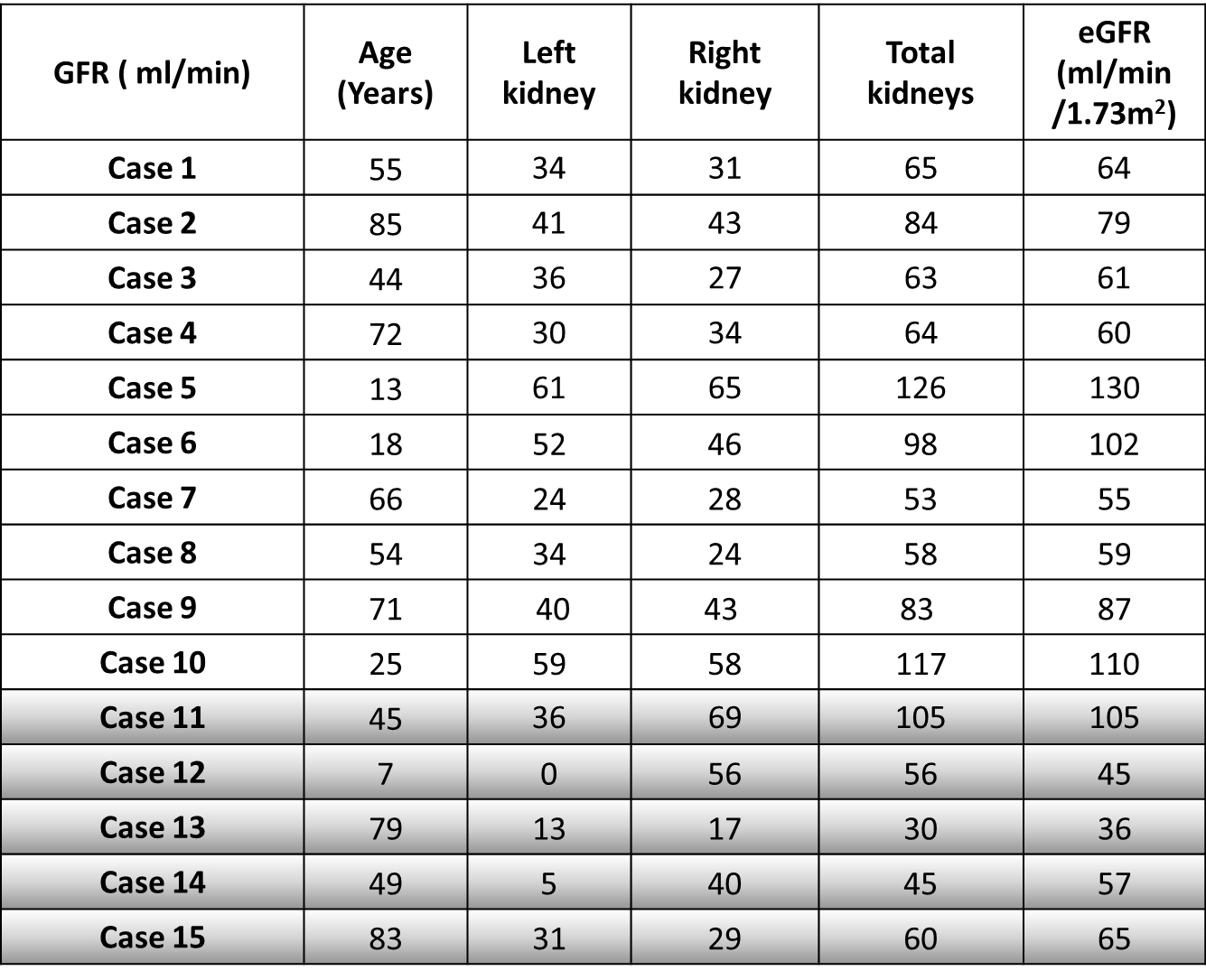
GFR estimates for the left and right kidneys estimated using the 4-sec temporal resolution CS reconstruction with the proposed HTR-AIF, for 15 patients are shown in Table 1. The total GFR values closely match eGFR calculated using serum creatinine values, validating the quantitative accuracy of our method. There was no statistically significant difference between MRI based total GFR and serum creatinine based eGFR estimates (p <0.05).

Conclusion:

Acknowledgements

References

[1] Pandey, A., Yoruk, U., Sharma, P., Martin, M.R., Altbach, M.I., Bilgin, A., Saranathan, M., Multiresolution imaging using golden angle stack-of-stars and compressed sensing. In: Proceedings of International Society for Magnetic Resonance in Medicine (ISMRM), Singapore 2016. (Abstract #0702).

[2] Yoruk, U., Saranathan, M., Loening, A. M., Hargreaves, B. A. and Vasanawala, S. S. (2015), High temporal resolution dynamic MRI and arterial input function for assessment of GFR in pediatric subjects. Magn Reson Med. doi: 10.1002/mrm.25731.

[3] Altbach MI, Bilgin A, Li Z, Clarkson EW, Trouard TP, Gmitro AF, Processing of radial fast spin-echo data for obtaining T2 estimates from a single k-space data set. Magn Reson Med 2005; 54: 549–559.

[4] Feng, L., Grimm, R., Block, K. T., Chandarana, H., Kim, S., Xu, J., Axel, L., Sodickson, D. K. and Otazo, R. (2014), Golden-angle radial sparse parallel MRI: Combination of compressed sensing, parallel imaging, and golden-angle radial sampling for fast and flexible dynamic volumetric MRI. Magn Reson Med, 72: 707–717. doi: 10.1002/mrm.24980.

[5] Tofts PS, Cutajar M, Mendichovszky IA, Peters AM, Gordon I (2012) Precise measurement of renal filtration and vascular parameters using a two-compartment model for dynamic contrast-enhanced MRI of the kidney gives realistic normal values. Eur Radiol 22:1320–1330.

[6] Delanaye P, Schaeffner E, Ebert N, et al. Normal reference values for glomerular filtration rate: what do we really know? Nephrol Dial Transplant 2012; 27: 2664–2672.