0777

From Visualization to Quantification: Calibrating Motion Magnification by Amplified Magnetic Resonance Imaging

Wendy W Ni¹, Maged Goubran¹, Greg Zaharchuk¹, Michael Moseley¹, Kristen Yeom¹, and Samantha Holdsworth¹

¹Radiology, Stanford University, Stanford, CA, United States

Synopsis

The brain is constantly in motion. Changes in the cardio-ballistic motion of brain structures can provide invaluable information on natural processes and pathology. We have previously introduced a qualitative visualization technique, Amplified MRI (aMRI), to amplify subtle cardio-ballistic motion in the brain. Now we attempt to quantify the underlying motion through simulation-based characterization of the aMRI technique. By generating calibration curves for a range of motion parameters, we calculated the unamplified tissue displacement in two human subjects. The estimated displacements are higher than literature values. Nevertheless, our simulations are the first steps in benchmarking aMRI’s potential as a quantitative technique.

Purpose

Natural processes and pathology can alter cardio-ballistic motion of brain structures ¹. To visualize these often sub-voxel motions, we have previously introduced amplified Magnetic Resonance Imaging (aMRI) ² to amplifies these motions. In this study, we add quantitative capability to aMRI using a simulation-based calibration of the apparent motion amplification, so that we can calculate the underlying tissue displacement.

Methods

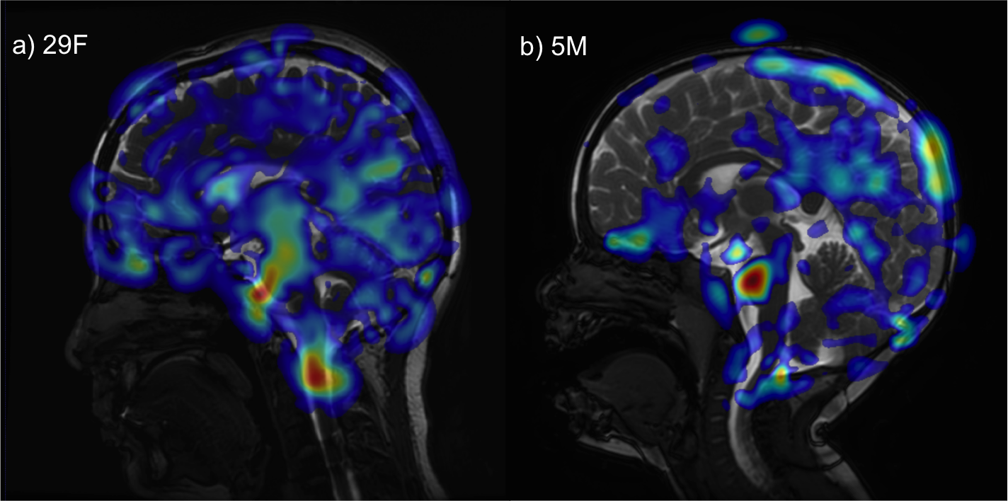
In vivo imaging: As described in Holdsworth et al. ², we acquired a 2D mid-line sagittal slice in 2 subjects (1 adult healthy volunteer, 29yrF; 1 pediatric patient with no known brain abnormality, 5yrM) using a cardiac-gated balanced steady-state free precession (bSSFP) sequence (matrix size 224×224 and reconstructed with zero-filling to 512×512, flip angle 45°, TR/TE 3.6/1.3ms; FOV 24mm²; slice thickness 4mm, acceleration factor 2, peripheral cardiac gating, retrospective re-binning to 150 cardiac phases. 1 view/segment and scan time 3min30sec [adult], and 6 views/segments and scan time 50sec [pediatric]). Eulerian Video Magnification (EVM) ³ was implemented in MATLAB (MathWorks, Natick MA) and run with parameters $$$\alpha=25$$$ and $$$\lambda_c=8(1+ \alpha)×0.14$$$mm, and a temporal bandpass filter chosen to selectively amplify the 2^nd to 4^th harmonics ².

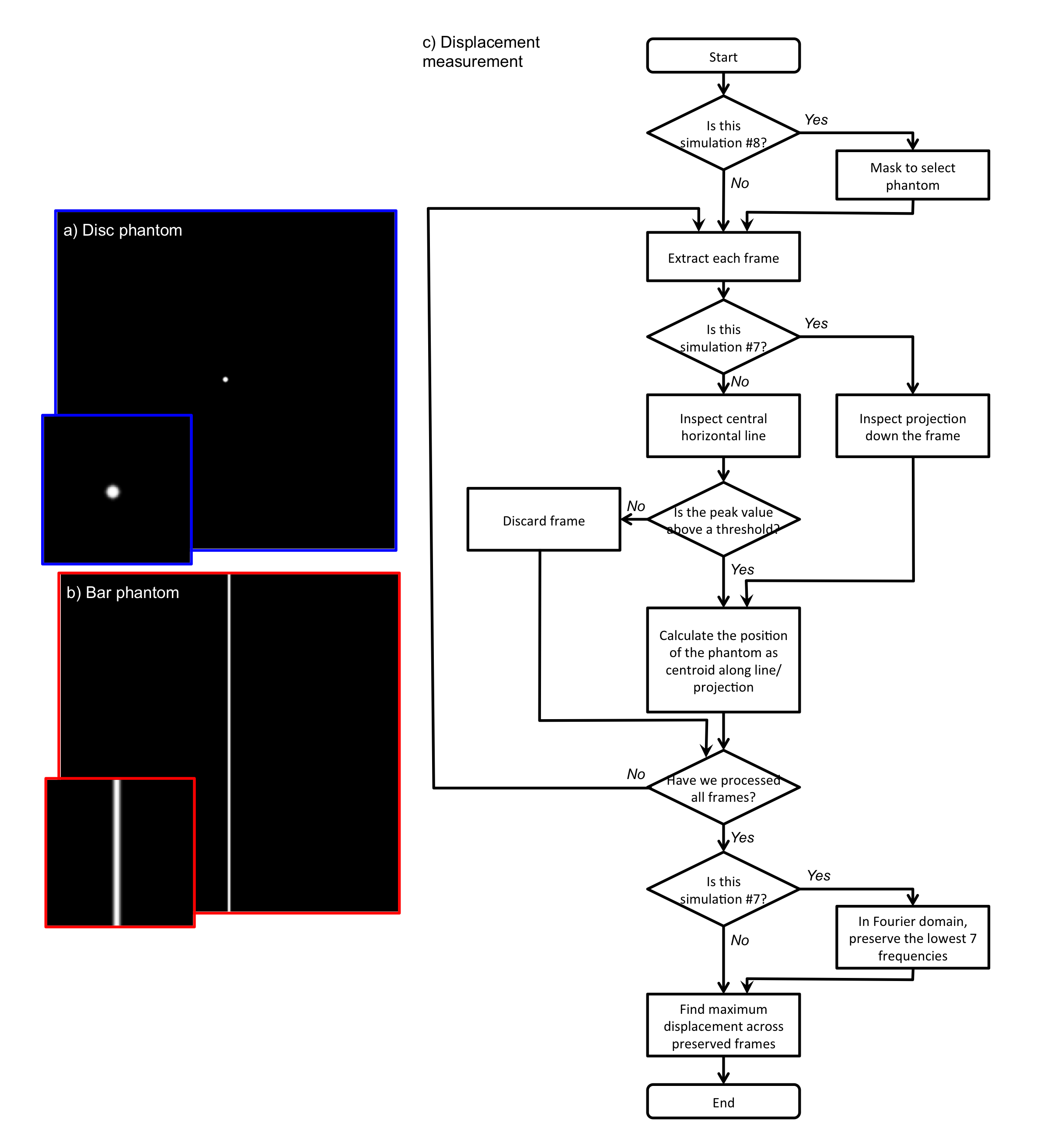
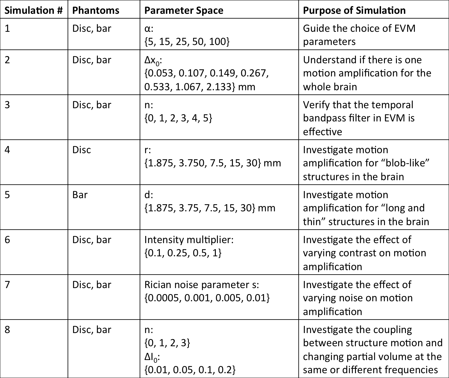
Simulation: We simulated aMRI in MATLAB, using two 2D digital phantoms (intensity 1 on background intensity 0, blurred with a Gaussian filter with FWHM of 2 voxels): a disc with radius $$$r$$$, and a vertical bar with width $$$d$$$ (Figure 1). The disc was chosen to emulate a generic moving “blob”, and the latter to emulate the bright CSF around the midbrain and spinal cord. Each digital phantom was translated with 1D sinusoidal displacement $$$\Delta x=\Delta x_0*sin(2n\pi t/150)$$$, with amplitude $$$\Delta x_0$$$, harmonic number $$$n$$$, and phase $$$t$$$. We investigated the coupling between motion and partial-volume changes by adding a 2nd-harmonic intensity variation $$$\Delta I=\Delta I_0*sin(4\pi t/150)$$$ in addition to motion. We also tested noise-robustness by adding Rician noise with parameter $$$s$$$ to the digital phantoms. All simulations are described in full in Table 1. After performing EVM, the maximum amplified displacement $$$\Delta x_{aMRI}$$$ (half of amplified peak-to-peak distance) of the digital phantoms were measured using a custom algorithm (Figure 1), and divided by the known $$$\Delta x_0$$$ to generate the apparent motion amplification factor $$$\Delta x_{aMRI}/\Delta x_0$$$, so that calibration curves could be obtained.

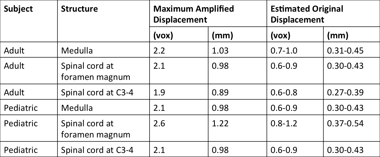
Verification: Using the calibration curves and manually measured maximum anterior-posterior displacements of the medulla, the spinal cord at the foramen magnum, and the spinal cord at C3-4 level on the in vivo images, we estimated the corresponding underlying tissue displacements.

Results

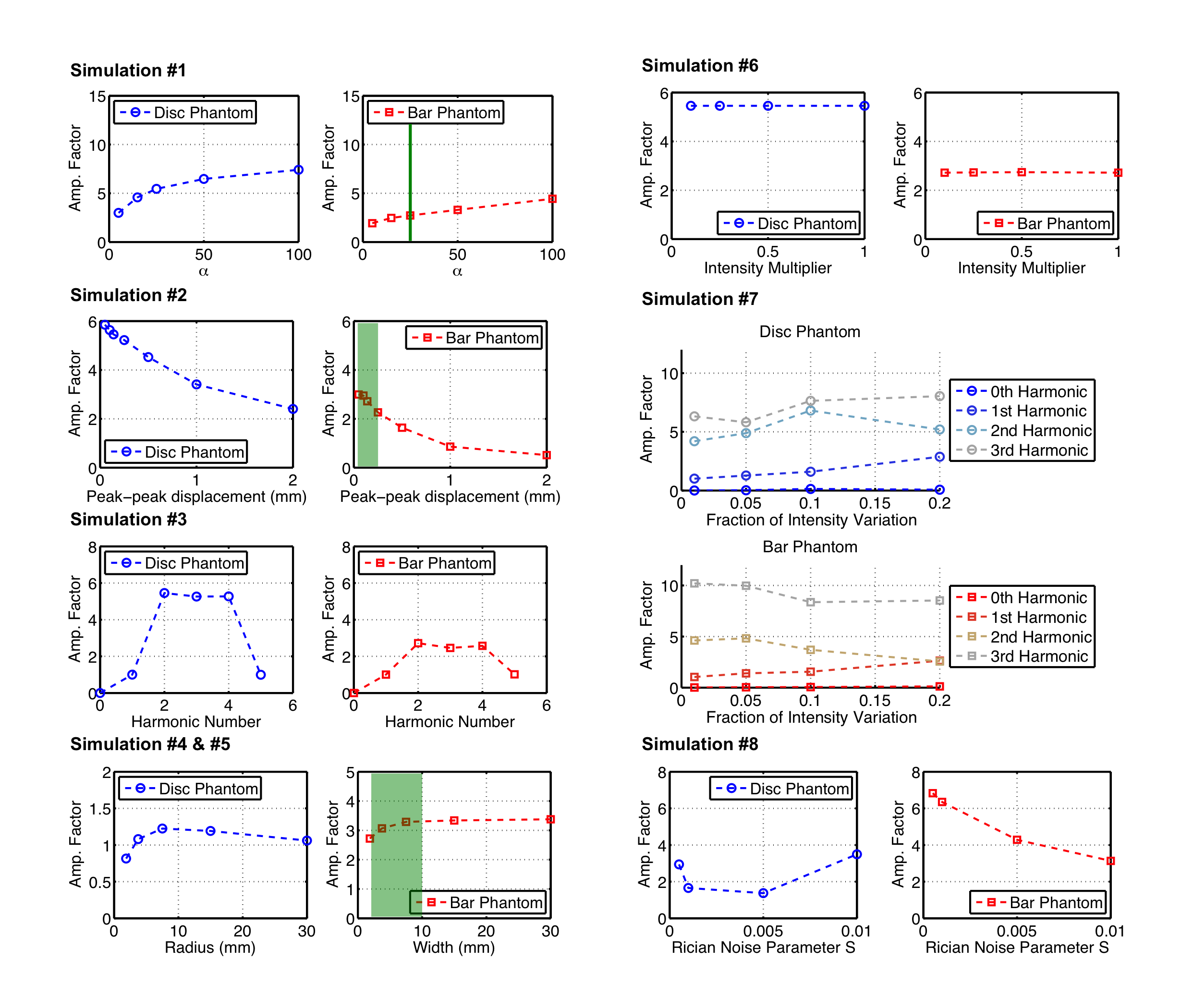
As shown in Figure 2, non-linear relationships exist between the amplification factor and all simulation variables. The choice of phantom also affected amplification. Because our simulated results have shown such complex interactions between the various parameters of the input images, and the amplification factor itself is displacement-dependent, we can only identify a range of motion amplification factors for verification, based on simulations #2 and #5. For our structures of interest, we expect peak-to-peak displacements of 0.05-0.25mm ⁴, and bright CSF “bar” widths of 2-10mm. Therefore, the amplification factors are around 2.3-3.3, and we estimated the unamplified displacement to be 0.27-0.54mm (Table 2).

Discussion

Simulation #3 and #6 support our expectations that the temporal bandpass filter is effective, and that overall image contrast does not affect motion amplification. However, the strong non-linearity shown in simulations #1, #2, #4, #5 and #8 poses a significant problem for aMRI’s application as a quantitative technique. In particular, the dependence of amplification factor on displacement introduces ambiguity into the process of converting amplified displacement back to the underlying displacement.

Using our estimated range of amplification factors, we find overestimation of midbrain and spinal cord motion in comparison to literature. From Simulation #8, we see that motion-independent intensity variation, such as changing partial volume effects, can significantly increase the apparent motion amplification factor, which may partially account for the overestimation.

Furthermore, our displacement measurement algorithm did not demonstrate stable performance with noisy images, which may have led to the noise-dependent amplification shown in simulation #7, thus we need to further refine the algorithm. We are investigating an alternative algorithm based on non-rigid body image coregistration, and have generated preliminary in vivo images in Figure 3.

Conclusion

This study is the first quantitative analysis ofaMRI, and provides valuable information on whether and how aMRI can be used to estimate actual brain structure displacement. Future work will include more simulations with denser coverage of the parameter space, digital phantom designs to emulate more complex brain structures (e.g. cerebellum), and better displacement measurement algorithms for both digital phantoms and in vivo images.

Acknowledgements

NIH NCRR 5P41RR09784. GE Healthcare. Stanford-Philips Research Agreement: Advancing Precision Health.

References

1. Greitz et al., Neuroradiology, 1992;34:370–380.

2. Holdsworth et al., Magn. Reson. Med., 2016 (in press).

3. Wu et al., ACM Trans. Graph., 2012;31:1–8.

4. Enzmann et al., Radiology 1992;185:653–660.

Figures

Figure 1: Digital phantoms used in simulation: a) disc phantom with radius $$$r$$$ of 4 voxels (1.875 mm) and low-passed with a Gaussian filter with FWHM 2 voxels; b) bar phantom with width $$$d$$$ of 4 voxels (1.875 mm) and low-passed with the same Gaussian filter. Insets show magnified view of the central region of the digital phantoms. c) Flow chart of the algorithm used to determine the amplified displacement $$$\Delta x_{aMRI}$$$ of digital phantoms in aMRI simulations. Simulations are described in detail in Table 1.

Table 1: Due to the large parameter space, we performed selected simulations to investigate various aspects of the aMRI method with potential impact on clinical use.

Figure 2: Summary of simulation results. Note that we are covering the simulation parameter space quite sparsely due to the large number of variables. For verification using realistic images, we are estimating the motion amplification factor using simulations #2 and #5, with the expected in vivo parameter ranges highlighted in green. The green line in simulation #1 indicates the actual value of α used for the in vivo images.

Table 2: Manual measurements of maximum amplified displacement from in vivo images, and corresponding ranges of estimated unamplified displacements of various brain structures.

Figure 3: Preliminary results from a non-rigid body coregistration-based method of automatically quantifying displacement in the two in vivo datasets. The color overlay is a measure of average displacement per cardiac phase. Quantitation is still in progress, but the locations of high-displacement regions correspond to visual inspection and manual measurements.

Proc. Intl. Soc. Mag. Reson. Med. 25 (2017)

0777