0774
Improved Short-T2* Estimation with Bloch Equation-Modeled Concurrent Excitation and Relaxation1Electrical Engineering, Stanford University, Stanford, CA, United States, 2Radiology, Stanford University, Stanford, CA, United States
Synopsis
Short-T2* magnetization (order of [0.1,1ms]) can relax appreciably during standard-rate excitation pulses, which can bias estimates of relaxation rates formed by fitting to observed signal decay. The effect can, however, be included in an updated model to improve T2* estimation for fast-relaxing signals. Here, a demonstration is presented.
Purpose
Measurements or estimations of $$$R_2^*$$$ (or $$$R_2$$$) values from MRI traditionally are formed from a series of images acquired at different echo times. The echo train documents signal decay, to which an exponential function can be fit and from which $$$R_2^*$$$—the decay rate—estimated. This typically does not incorporate accounting for relaxation occurring during the excitation pulse, as for the $$$R_2^*$$$ ranges (order of [10,100]ms) observed in many tissues it is insignificant. However, for some, e.g., cortical bone, intra-excitation relaxation can be non-negligible[1–3]. If ignored, it can bias estimates; but if considered, it can be leveraged, facilitating improved $$$R_2^*$$$ estimation. Here, a description and demonstration of accounting for this phenomenon to better estimate relaxation rates in short-$$$T_2^*$$$/high-$$$R_2^*$$$ (order of [0.1,1]ms) signals is presented.Theory
Conventional $$$R_2^*$$$ estimation proceeds by fitting signal progressions acquired over collected echo times $$$\{t_i\}_i$$$ to a model of the form$$f(R_2^*,t_i;\gamma)=g(\gamma)\exp(-{R_2^*}{t_i})\textrm{,}$$where $$$g(\gamma)$$$ is some function describing sequence-determined signal-amplitude dependence upon assumed-known parameters—e.g., tip angle $$$\alpha$$$, repetition time TR—and may include co-estimation parameters—e.g., equilibrium magnetization $$$M_0$$$[4,5]. In terms of $$$R_2^*$$$, $$$f$$$ is a decaying exponential. The fit can be formed by constrained minimization of the squared error between modeled signal and measured signal (C-L-S; also called 'non-linear least-squares' or NLLS)[4,6].
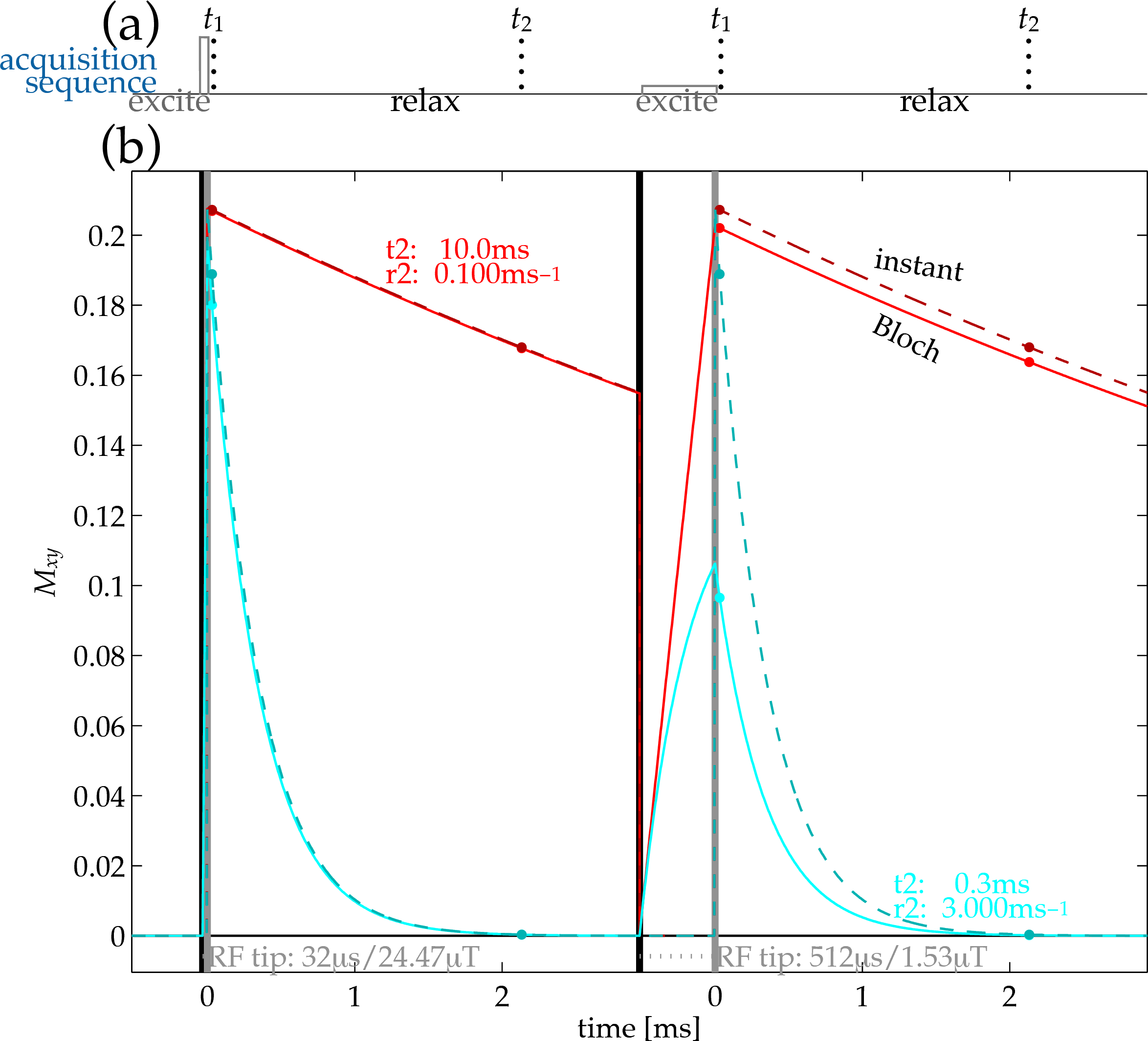
If $$$R_2^*$$$ is significant relative to the $$$B_1$$$ excitation rate, appreciable relaxation occurs during the excitation[3,7,8]. This suggests manipulating excitation amplitude $$$B_1$$$ as a complementary mode of interrogating relaxation. Using the Bloch equation to calculate the effect leads to an update of the fitting model to one of the form$$f(R_2^*,t_i,(B_1,\alpha);\gamma)=\tilde{g}(\gamma)b(R_2^*,B_1,\alpha)\exp(-{R_2^*}{t_i})\textrm{,}$$where $$$b(R_2^*,B_1,\alpha)$$$ describes the Bloch-simulated excitation (Fig.1).
Methods
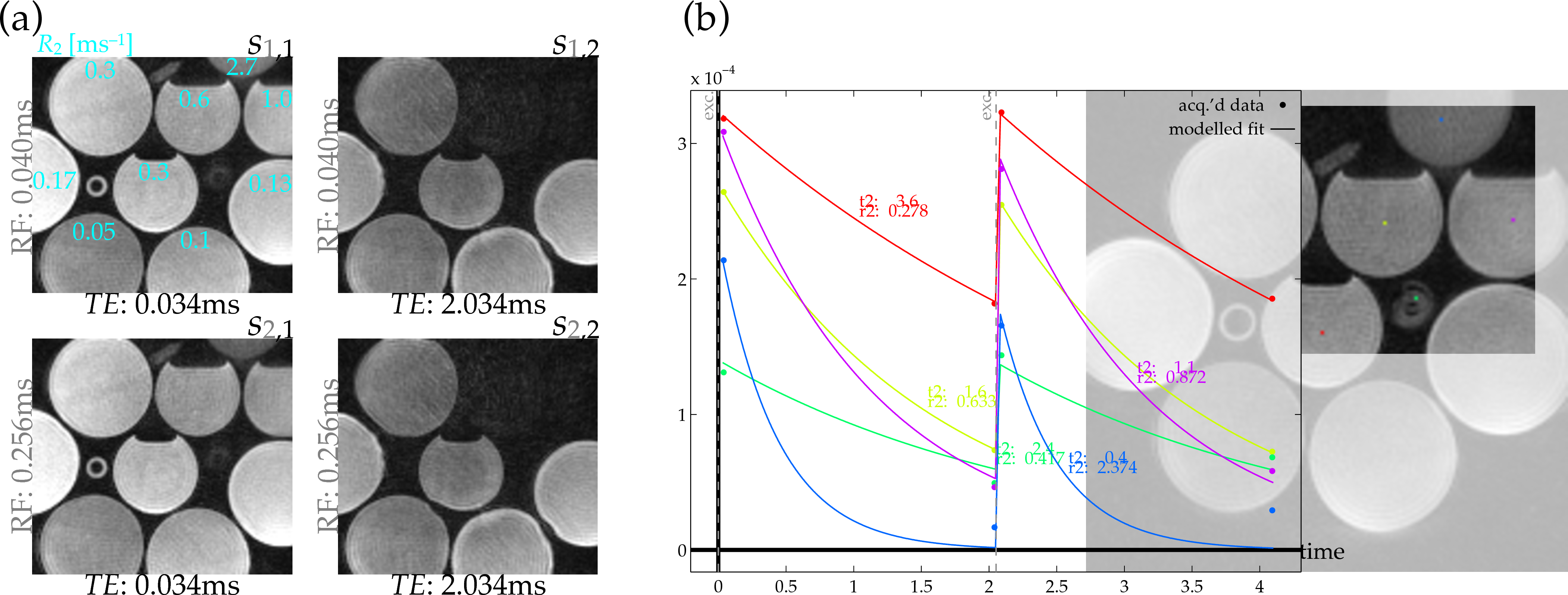
Images of bottle phantoms and rubber structures (Fig.2) were acquired by a dual-echo/dual-excitation 3D UTE sequence (Fig.1), recording four images from each pairing of RF-excitation rate (15$$$^{\circ}$$$ tip at 24.47μT or 3.8228μT) and echo time (40μs or 2.04ms). Bottles contained MnCl$$$_{\textrm{2}}$$$-doped water varied in concentrations, creating a range of different $$$R_2^*$$$ relaxation rates (Fig.2) Exact $$$R_2^*$$$ values in the rubber compounds are unknown, but they are expected to be high (1ms$$$^{-\textrm{1}}$$$ or higher)[9]. The spoiled gradient-echo sequence acquired with (1.25mm)$$$^{\textrm{3}}$$$ resolution at 9$$$\times$$$ undersampling with 6.4ms TR from a 1.5T scanner with an eight-channel receive-only head coil/body transmit coil.
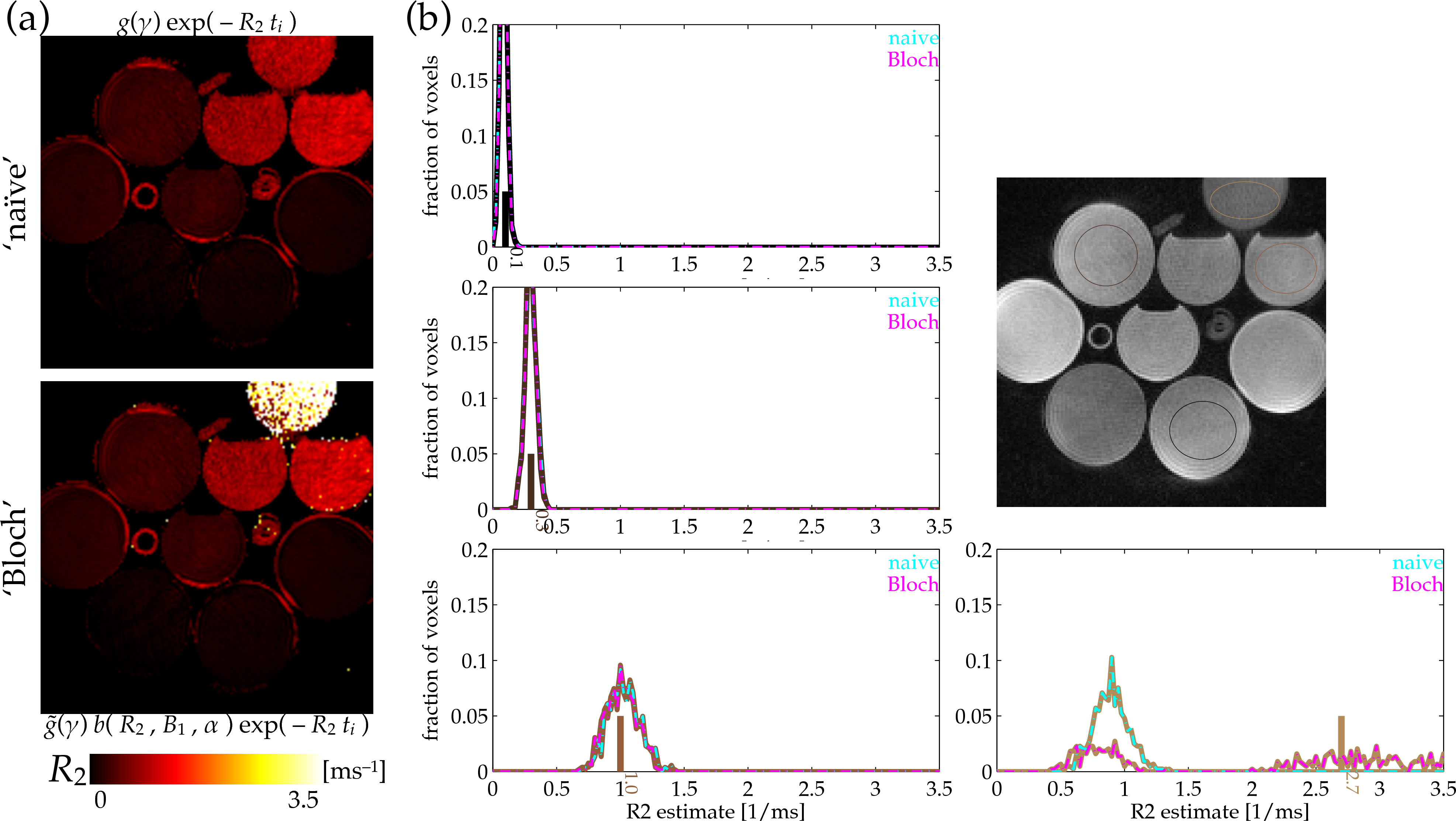
Estimating $$$R_2^*$$$ was undertaken by C-L-S with a soft-baseline function accounting for magnitude/Rician noise[10]. This does not provide the maximum likelihood estimate, but it can perform well[4,5]. This approach is the same as C-L-S used in 'traditional' $$$R_2^*$$$ estimation, except that its signal model is updated to include the Bloch-simulation factor $$$b(R_2^*,B_1,\alpha)$$$. Equilibrium magnetization $$$M_0$$$ was jointly estimated. Voxels with smaller-than-5%-maximum $$$M_0$$$ estimates were masked to 0 in displayed $$$R_2^*$$$ maps (Fig.3).
Results
Estimates of $$$R_2^*$$$ formed 'naively' without accounting for the excitation rate (top-left) give relatively accurate $$$R_2^*$$$ estimates in longer-$$$T_2^*$$$ phantoms, but they fail to distinguish the $$$R_2^*$$$ values in shorter-$$$T_2^*$$$ bottle phantoms (Fig.3). Accounting for the excitation-concurrent relaxation using a Bloch simulation fit corrects estimates of the short-$$$T_2^*$$$-phantoms relaxation rates (Fig.3). E.g., estimates in the high-, 2.7ms$$$^{-\textrm{1}}$$$ $$$R_2^*$$$ phantom formed by naive estimation are biased even below the 1ms$$$^{-\textrm{1}}$$$-phantom estimates (Fig.3:cyan-dashed-tan population), while Bloch-fit estimates (Fig.3:magenta-dashed-tan population) are localized in the correct regime. Although the estimate variance is much higher, it is not biased away from the true value (Fig.3:short, solid tan line) as it otherwise was.Discussion
Estimating $$$R_2^*$$$ is challenging because the exponential decay curve is a relatively 'weak' basis function, in that all decay rates induce the same shape of signal progression. Interrogating signals using different rates of excitation facilitates some easement of the estimation problem in this sense by generating a set of measurements that are 'more orthogonal'. This allows better distinction of short-$$$T_2^*$$$ signals in particular and can improve estimation accuracy. However, making precise estimates of short-$$$T_2^*$$$ signals is still challenging, because with faster decay they effectively permit fewer sampling opportunities. For example, while a moderate-$$$T_2^*$$$ signal acquired using two excitation rates and sampled at two echo times yields four non-zero measurements, a short-$$$T_2^*$$$ (relative to the later echo times) signal yields only two.
The analysis presented here assumes mono-exponential decay (i.e. single-$$$T_2^*$$$-value) in all voxels. In some cases the assumption may not hold; however, with adequate measurements, the same approach—incorporating intra-excitation relaxation effects—can be employed with other, multi-component models.
Conclusion
For relaxometry of objects creating short-$$$T_2^*$$$ signals, accounting for intra-excitation relaxation through Bloch-equation signal modeling improves short-$$$T_2^*$$$ estimates ($$$T_2^*$$$ $$$\sim$$$ [0.1,1]ms). The Bloch modeling turns a source of systematic bias into a complementary measurement, facilitating short-$$$T_2^*$$$ signal interrogation through manipulation of $$$B_1$$$. This does not affect estimation with longer-$$$T_2^*$$$ ($$$\sim$$$ [10,100]ms) signals.Acknowledgements
NIH P01 CA159992 and P41 EB015891References
[1] Larson, P. E., Gurney, P. T., Nayak, K., Gold, G. E., Pauly, J. M., & Nishimura, D. G. (2006). Designing long-T2 suppression pulses for ultrashort echo time imaging. Magnetic resonance in medicine, 56(1), 94-103.
[2] Du, J., Carl, M., Bydder, M., Takahashi, A., Chung, C. B., & Bydder, G. M. (2010). Qualitative and quantitative ultrashort echo time (UTE) imaging of cortical bone. Journal of Magnetic Resonance, 207(2), 304-311.
[3] Johnson, E. M., Vyas, U., Ghanouni, P., Pauly, K. B., & Pauly, J. M. (2016). Improved cortical bone specificity in UTE MR Imaging. Magnetic resonance in medicine.
[4] Hernando, D., Kramer, J. H., & Reeder, S. B. (2013). Multipeak fat-corrected complex R2* relaxometry: Theory, optimization, and clinical validation. Magnetic resonance in medicine, 70(5), 1319-1331.
[5] Ghugre, N. R., Enriquez, C. M., Coates, T. D., Nelson, M. D., & Wood, J. C. (2006). Improved R2* measurements in myocardial iron overload. Journal of Magnetic Resonance Imaging, 23(1), 9-16.
[6] Hernando, D., Liang, Z. P., & Kellman, P. (2010). Chemical shift–based water/fat separation: A comparison of signal models. Magnetic resonance in medicine, 64(3), 811-822.
[7] Carl, M., Bydder, M., Du, J., Takahashi, A., & Han, E. (2010). Optimization of RF excitation to maximize signal and T2 contrast of tissues with rapid transverse relaxation. Magnetic resonance in medicine, 64(2), 481-490.
[8] Springer, F., Steidle, G., Martirosian, P., Claussen, C. D., & Schick, F. (2010). Effects of in-pulse transverse relaxation in 3D ultrashort echo time sequences: analytical derivation, comparison to numerical simulation and experimental application at 3T. Journal of Magnetic Resonance, 206(1), 88-96.
[9] Robson, M. D., Gatehouse, P. D., Bydder, M., & Bydder, G. M. (2003). Magnetic resonance: an introduction to ultrashort TE (UTE) imaging. Journal of computer assisted tomography, 27(6), 825-846.
[10] Gudbjartsson, H., & Patz, S. (1995). The Rician distribution of noisy MRI data. Magnetic resonance in medicine, 34(6), 910-914.
Figures