0752

Spatiotemporal analysis of breathing-induced fields in the cervical spinal cord at 7T

S. Johanna Vannesjo¹, Karla L. Miller¹, Stuart Clare¹, and Irene Tracey¹

¹FMRIB centre, Nuffield Department of Clinical Neurosciences, University of Oxford, Oxford, United Kingdom

Synopsis

Time-varying B₀ fields related to breathing is one major source of image artifacts in spinal cord imaging at ultra-high field. Here we aim to measure spatial and temporal characteristics of breathing-induced fields in the cervical spinal cord at 7T. We perform a principal component analysis on field measurements based on fast gradient-echo images acquired during free breathing. We observed field variations of about 30Hz at C7 during normal breathing. Furthermore, we observed that a single principal component explained over 90% of the field variance during normal and deep breathing.

Purpose

To investigate spatial and temporal characteristics of respiratory-induced B₀ fields in the cervical spinal cord during free breathing.

Introduction

Spinal cord imaging would benefit from going to ultra-high field, as the increased SNR enables higher image resolution and thus more accurate depiction of fine anatomical details. However, several technical challenges are exacerbated at ultra-high field. Specifically, time-varying B₀ fields related to the changing lung volume and chest motion during the breathing cycle is one major source of image artifacts, resulting for example in ghosting and time-varying apparent motion.

A first step towards addressing the issue is to characterize the spatial and temporal characteristics of the breathing-induced fields. The spatial distribution has previously been investigated at 3T ¹ and at 7T ², by comparing B₀ field maps acquired during inspired or expired breath-holds. This however does not capture the temporal dimension of the field variations. In this work, we use fast gradient-echo acquisitions to measure respiratory field fluctuations during free breathing in the cervical spinal cord at 7T. Subsequently, we apply a principal component analysis to evaluate spatiotemporal characteristics.

Methods

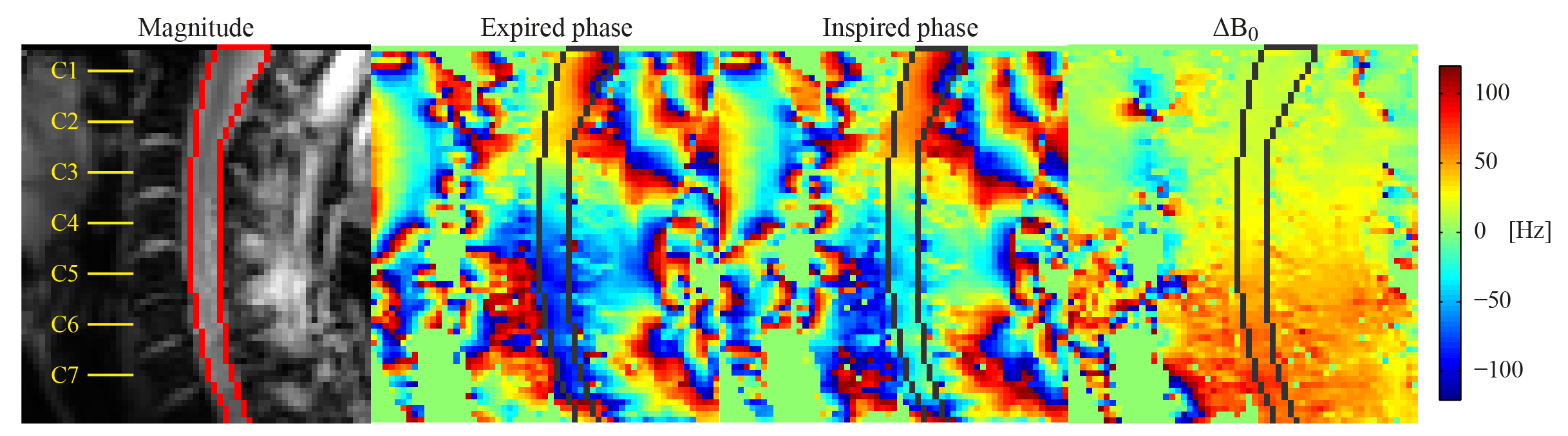
Imaging was performed in six healthy volunteers (3 male) on a whole-body 7T system (Magnetom, Siemens Healthcare), using a volume-transmit 16-channel receive cervical spine coil (Quality Electrodynamics). Fast gradient echo acquisitions (FOV 144x144mm², resolution 3.4x2.3mm², slice thickness 3mm, TE 4.08ms, TR 8ms, FA 6˚, volume TR 344ms) of a single sagittal slice through the center of the spinal cord were acquired (Fig. 1). During acquisitions the subjects were instructed to breathe normally, breathe deeply or perform inspired/expired breath-holds.

The phase of each voxel was unwrapped over time, and the mean phase offset was subtracted to remove phase contributions from static B₀ and B₁. Time-varying B₀ fields were subsequently obtained as $$$\Delta B_0({\bf r} ,t)=\frac{\phi({\bf r} ,t)}{2\pi TE} $$$. A mask covering the spinal cord was manually defined, and the field in voxels inside the mask was averaged at each position in the foot-head direction, yielding the field offset, $$$\Delta B_0(z,t)$$$.

A principal component analysis (PCA) was performed on $$$\Delta B_0(z,t)$$$ for 30s of acquisition in each of the breathing patterns, yielding a set of spatial principal components (PC), each related to one projection time course. Scaling the first PC with the peak-to-peak variation in the projection yielded an estimate of the magnitude of field variations for each subject and breathing pattern.

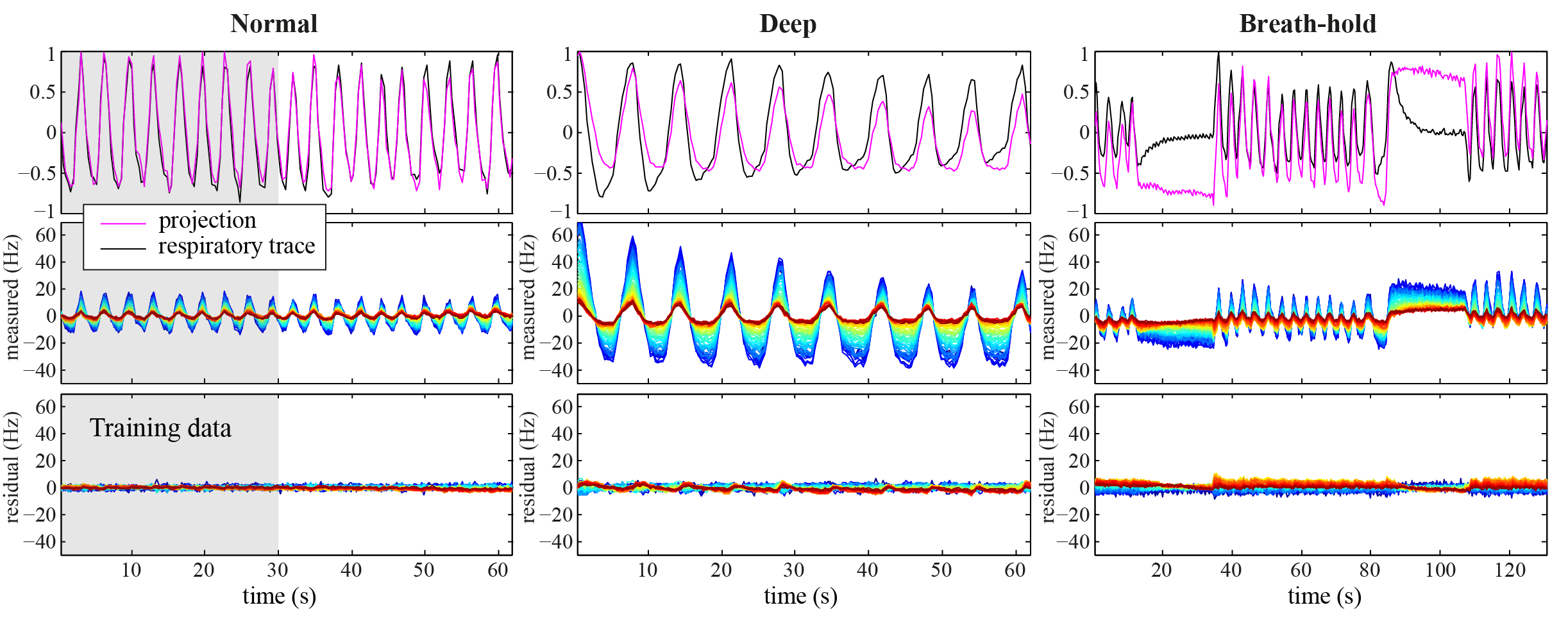
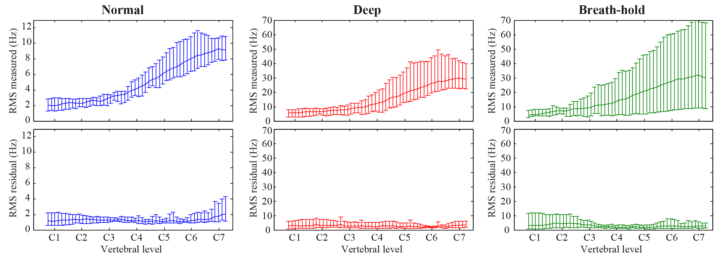
In order to assess the feasibility of implementing correction methods based on a PCA of training data, the measured $$$\Delta B_0(z,t)$$$ of all breathing patterns was projected onto the first PC of normal breathing, and the residual was quantified.

Results

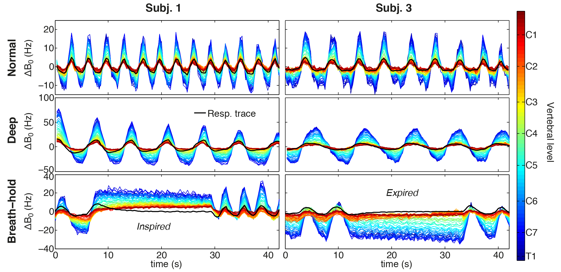
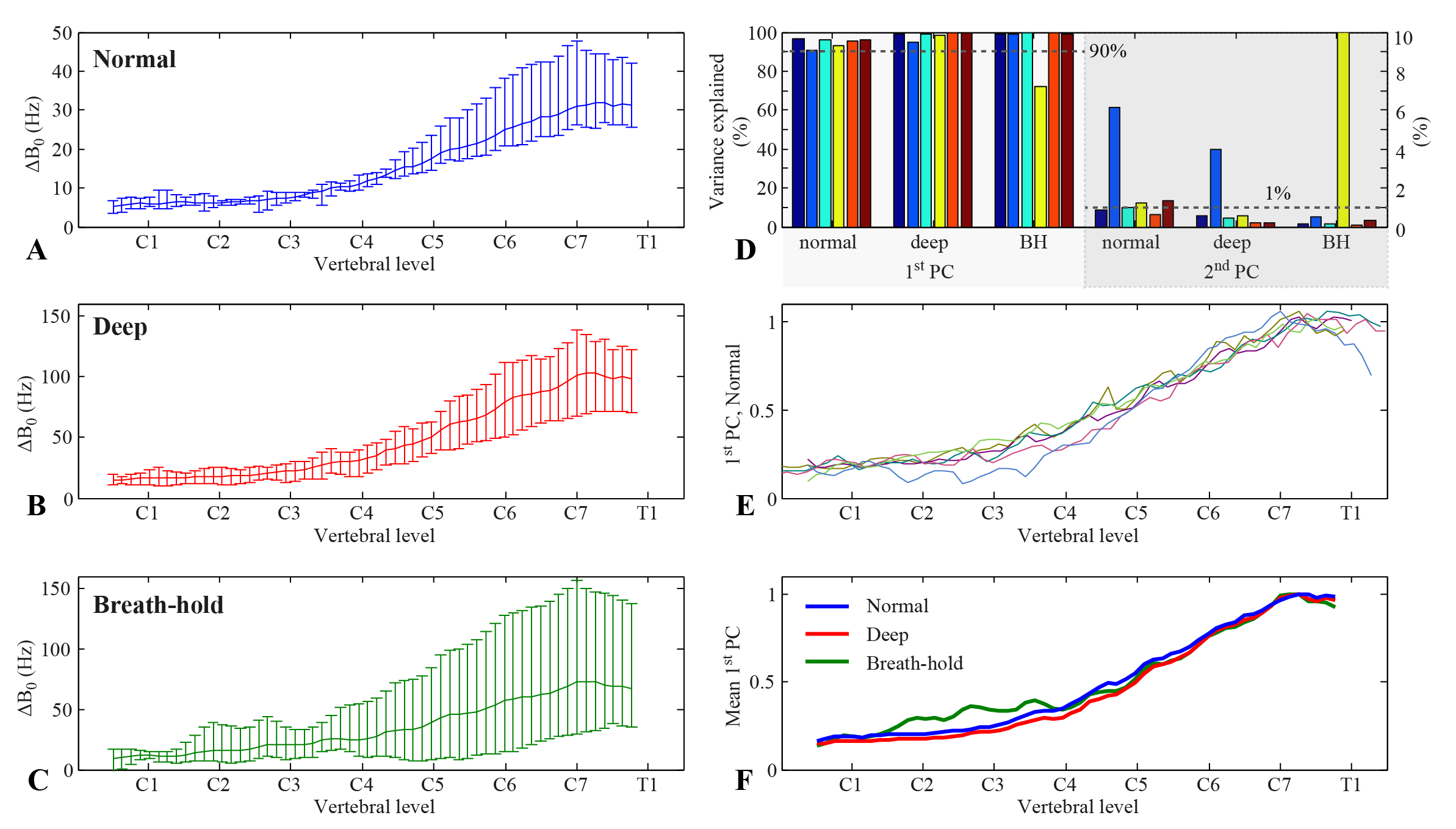
Figure 2 shows measured $$$\Delta B_0(z,t)$$$ during normal breathing, deep breathing and breath-holds. Peak-to-peak variations in the field at the level of C7 averaged around 31Hz and 103Hz for normal and deep breathing, respectively (Fig. 3A,B). Breath-hold acquisitions showed the largest variability between subjects (Fig. 3C). The first PC explained above 90% of the variance in all subjects and breathing patterns, except for breath-holds in one subject, whereas the second PC explained 1% or less in most cases (Fig. 3D). The first PC showed a high degree of similarity between subjects (Fig. 3E), and the mean PC over subjects was near identical between normal and deep breathing (Fig. 3F). In agreement with this, the first PC of normal breathing largely explained the field variations in all breathing patterns (Fig. 4), and the root-mean-square (RMS) of the residual was considerably reduced as compared to the original measured data, especially in lower parts of the cervical spine (Fig. 5).

Discussion and Conclusions

Here we have presented measurements of breathing-induced fields in the spinal cord under realistic conditions. We observed field variations of about 30Hz at C7 during normal breathing. This is considerably lower than previously reported values obtained from breath-hold measurements, which indicated field shifts at C7 of about 70Hz at 3T ¹ and 120Hz at 7T ². Breath-hold measurements in this work resembled deep breathing in magnitude, but with large variability between subjects.

We observed that a single principal component explains over 90% of the field variance during normal and deep breathing, and that training data from normal breathing can largely capture subsequent field variations of different breathing patterns. Correction methods could thus potentially make use of this feature, by relating measured fields from a training dataset to an external tracker of the current breathing state. Similar approaches have been implemented for brain imaging at ultra-high field by applying compensation shim fields in real-time based on signal from a respiratory bellow³ or field probes⁴.

Acknowledgements

This project has received funding from the Wellcome Trust Strategic Award and from the European Union’s Horizon 2020 research and innovation programme under the Marie Sklodowska-Curie grant agreement No 659263.

References

1. Verma T, Cohen-Adad J. Effect of respiration on the B0 field in the human spinal cord at 3T. Magn Reson Med 2014;72:1629–1636.

2. Vannesjo SJ, Eippert F, Kong Y, Clare S, Miller KL, Tracey I. Breathing-induced B0 field fluctuations in the cervical spinal cord at 7T. ISMRM 2016. p. 49.

3. van Gelderen P, de Zwart JA, Starewicz P, Hinks RS, Duyn JH. Real-time shimming to compensate for respiration-induced B0 fluctuations. Magn Reson Med 2007;57:362–368.

4. Duerst Y, Wilm BJ, Dietrich BE, Vannesjo SJ, Barmet C, Schmid T, Brunner DO, Pruessmann KP. Real-time feedback for spatiotemporal field stabilization in MR systems. Magn Reson Med 2015;73:884–893.

Figures

Fig. 1: Sagittal single-slice acquisition used to measure field fluctuations during free breathing. Displayed are the mean magnitude image (left), phase images acquired during an expired and an inspired breath-hold (middle), and the difference between the two phase images (right), scaled to Hz. The outline of the spinal cord mask is overlaid on each image.

Fig. 2: Time-courses of measured breathing-induced field fluctuations during normal breathing, deep breathing, and breath-holds in two subjects. The line color indicates the vertebral level of the measured field offset. Overlaid in black is the simultaneously acquired trace from a respiratory bellow.

Fig. 3: Magnitude of field variations during A) normal breathing, B) deep breathing and C) breath-holds. The plots show the mean and range over all subjects. D) Variance explained by the first and second principal component in all subjects and breathing patterns. Note the different axes for the first and the second PC. E) The first principal component of normal breathing for all subjects. F) The mean of the first principal component over all subjects for normal breathing, deep breathing and breath-holds.

Fig. 4: Projections of measured $$$\Delta B_0(z,t)$$$ onto the first principal component of normal breathing. The top row shows the time-courses of the projections together with the trace from a respiratory bellows. The middle row shows the measured $$$\Delta B_0(z,t)$$$, and in the lower row are the residual errors after projection. The gray areas indicate the training dataset. The color scale of $$$\Delta B_0(z,t)$$$ is the same as in Figure 2.

Fig. 5: A) Root-mean-square (RMS) of the measured field fluctuations during normal breathing, deep breathing and breath-holds. B) RMS of the residual after projection onto the first principal component. The plots show the mean and ranges of the RMS values over all subjects.

Proc. Intl. Soc. Mag. Reson. Med. 25 (2017)

0752