0748
Understanding Reciprocity1Center for Advanced Imaging Innovation and Research (CAI2R) and Bernard and Irene Schwartz Center for Biomedical Imaging, Department of Radiology, New York University School of Medicine, New York, NY, United States, 2Sackler Institute of Graduate Biomedical Sciences, New York University School of Medicine, New York, NY, United States
Synopsis
The principle of reciprocity, as it applies to magnetic resonance, is both remarkably powerful and regrettably easy to misconstrue. As evidence of this fact, each of us with an interest in the operation of radiofrequency coils need only recall the time we have spent trying to understand, in our guts, the difference between transmit and receive sensitivity patterns. As a respectful supplement to Dr. Hoult’s seminal explications, we here provide a highly streamlined derivation, aimed at bolstering intuition, and offer a simple but fundamental mnemonic to keep your pluses and your minuses straight.
Introduction
Since Hoult’s seminal paper characterizing the signal-to-noise ratio of the nuclear magnetic resonance experiment appeared in 1976,1 the principle of reciprocity has been used almost universally to understand and compute receive sensitivity patterns for radiofrequency (RF) coils used in MR. Some confusion arose in the interpretation of reciprocity once magnetic field strengths rose enough for transmit and receive sensitivity patterns to deviate noticeably from one another. These deviations led some to question the applicability of the reciprocity principle at high frequency. In another seminal paper,2 Hoult laid this concern to rest, interpreting reciprocity carefully in the setting of a rotating frame of reference. He identifyed the transmit sensitivity pattern with the field component B1(+)=(B1x+iB1y)/2, and the receive sensitivity pattern with the oppositely-circulating component B1(-)=(B1x-iB1y)/2. The distinct character of B1(+) and B1(-) has been validated extensively in simulations and experiments3. However, the explanation for why transmit and receive sensitivities are associated with distinct field components continues to defy simple intuitions, not only for students but even for many experts in the field. Hoult’s mathematics, while undeniably correct, are dense. Here, in an attempt to bolster physical intuition, we derive the distinction between transmit and receive sensitivities is a few simple lines, and show how the opposite apparent precession sense associated with these sensitivities relates directly to the inductive nature of MR signal detection.Theory
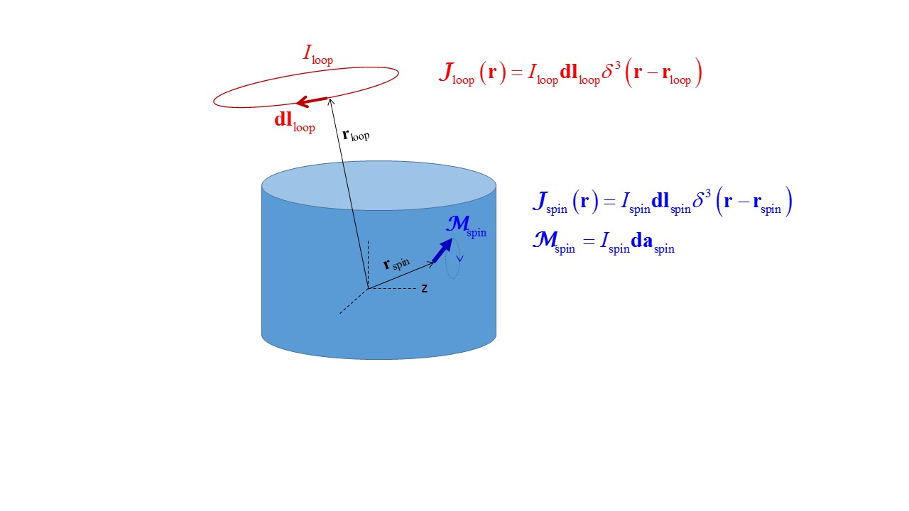
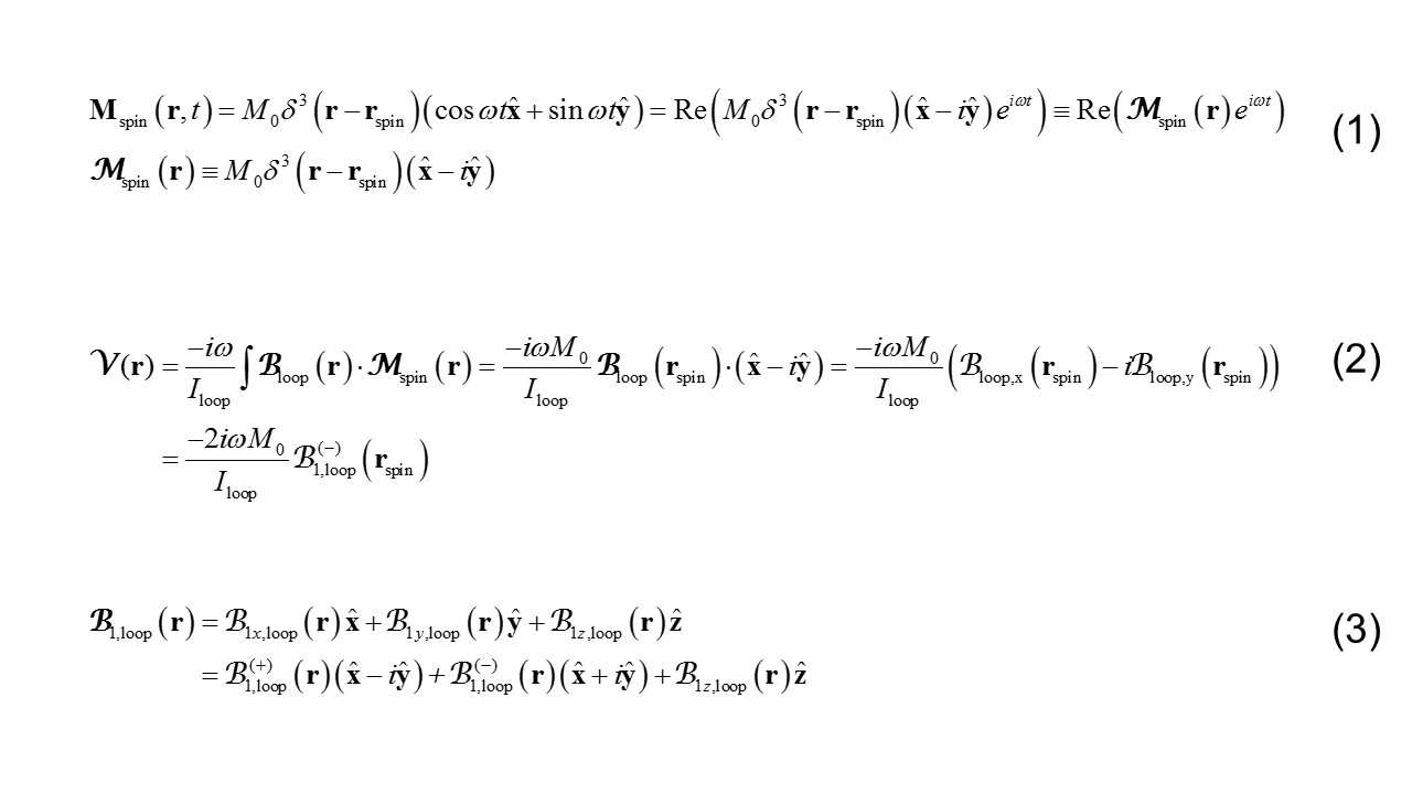
Figure 1 illustrates the geometry of our simple derivations to follow, in which an external conductive loop receives signal from a precessing spin embedded in a body. Figure 2 begins with an expression for the magnetic moment of the spin. In Equation 1, the real quantity Mspin(r,t) is expressed as the real part of a time-invariant complex moment multiplied by a harmonic time dependence with frequency ω (the Larmor frequency). This single convention for complex quantities will apply throughout. Positive precession of the spin magnetic moment is clearly associated with the complex combination of unit vectors x–iy.
Equation 2 begins with Hoult’s expression for the measured MR signal voltage1. The dot product of the loop’s magnetic field with the spin’s magnetic moment immediately identifies the signal sensitivity with B1(-).
Equation 3 simply decomposes the loop’s B1 field, originally expressed in Cartesian coordinates, into combinations involving x–iy and x+iy (leaving the details to be verified by the reader). The field coefficient co-rotating with the spin (i.e. sharing its x–iy directionality, and therefore stationary in its rotating frame) is obviously B1(+)!
In other words, the receive sensitivity is characterized by B1(-) because it results from a dot product with the spin magnetic moment, whereas the transmit sensitivity goes as B1(+) because the transmit field precesses with the spin magnetic moment.
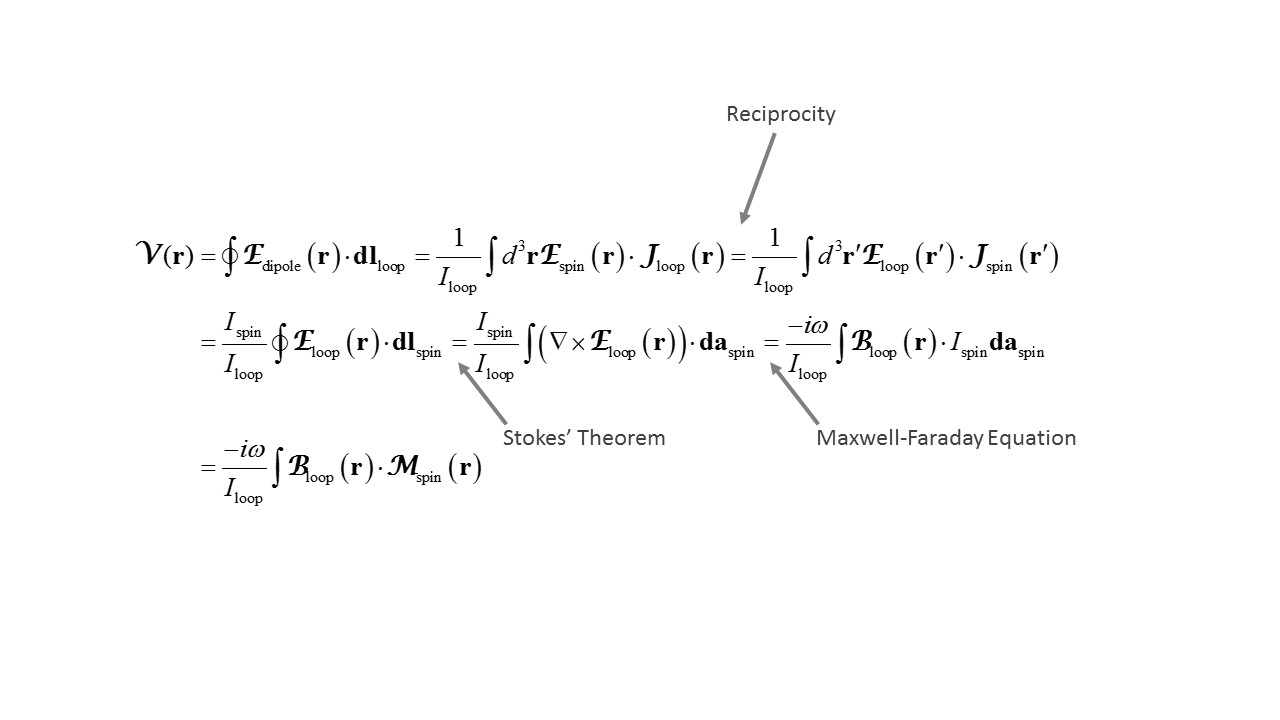
What is the origin of the dot product in the MR signal expression in Equation 2? Figure 3 contains a simple derivation of this expression, beginning from a definition of the signal voltage as an electromotive induced in the loop by the time-varying electric field of the precessing dipole. Reciprocity may then be applied in a traditional manner to exchange the E field and current density of the loop with that of the spin. Treatment of the spin as an equivalent infinitesimal current loop, followed by an application of Stokes’ Theorem and the Maxwell-Faraday Equation, yields Hoult’s original signal expression.
In short, the dot product derives directly from the inductive character of signal detection. When we measure an induced voltage or current in an RF coil, we are really measuring E∙dl, or J∙E , or B∙da. In signal reception, we are measuring the work done by the field of the precessing spin, whereas what matters for excitation is the field itself.
Discussion and Conclusions
This perspective on reciprocity is offered as a guide for students of MR, young and old, who wish to keep track of why signal reception should be associated with B1(-) and transmission with B1(+). The answer, in these terms, is simple: reception involves a dot product, and transmission does not.
This distinction, of course, may also be understood in more fundamental terms, with reference to creation and annihilation operators involving exchanges of energy from the coil to the spin and vice versa, or by analogy to the flip-flip term in the dipole-dipole coupling Hamiltonian, which takes a similar form. Not surprisingly, the ever-rigorous Dr. Hoult has explored such explanations as well.4 Let us close with one final question for the stout of heart: were a practical noninductive mechanism of routine MR signal detection to be devised5, what might its pattern of sensitivity be?
Acknowledgements
The Center for Advanced Imaging Innovation and Research (CAI2R, www.cai2r.net) at New York University School of Medicine is supported by NIH/NIBIB grant P41 EB017183.References
1. Hoult DI, Richards RE. The signal-to-noise ratio of the nuclear magnetic resonance experiment. J Magn Reson 1976;24:71-85.
2. Hoult DI. The Principle of Reciprocity in Signal Strength Calculations - A Mathematical Guide. Concepts Magn Reson 2000;12:173-187.
3. Collins CM, Yang QX, Wang JH, Zhang X, Liu H, Michaeli S, Zhu X-H et al. Different excitation and reception distributions with a single-loop transmit-receive surface coil near a head-sized spherical phantom at 300 MHz. Magn Reson Med 2002; 47(5): 1026-1028.
4. Hoult DI, Bhakar B. NMR signal reception: Virtual photons and coherent spontaneous emission. Concepts in Magnetic Resonance A 1997;9(5):277-297.
5. Hennig, JH. My dream high-field MR scanner. 2016 i2i workshop (www.cai2r.net/i2i).
Figures