Introduction

Simultaneous PET/MR is now being adapted for clinical studies. Previously, Dixon based LAVA-Flex MR images provided good soft-tissue contrast to characterize MR based PET attenuation map (MRAC), but bone was ignored. Development of UTE and zero-echo time (ZTE) MR imaging methods [1] have now enabled bone depiction in MR images. Most of previous methods (atlas, segmentation, machine learning) for incorporating bone in MRAC workflow considered all bones in the FOV as a single entity; irrespective of their density. In this work, we demonstrate using ZTE and Dixon LAVA-Flex MRI data, and deep learning framework, a continuous density pseudo-CT (pCT) image which combines soft tissue pCT (from Dixon LAVA-Flex) with a continuous density bone pCT from ZTE. Additional advantages include: common bone depiction framework and computational efficiency for deployment using pre-trained convolutional neural network model.

Methods and Materials

Patient data: Patients who underwent PET/CT scan were scanned in a TOF GE Signa PET/MR scanner. ZTE (proton density weighted) and Dixon LAVA-Flex images were acquired for head and pelvis. LAVA-Flex: head and pelvis, two-point Dixon, body transmit/receive coil, TE/TR=1.15ms-2.3ms/4.05ms, FA=5°, FOV=500×500×312mm3, resolution = 1.95mm×1.95mm×2.6mm. Fat and water images were reconstructed from LAVA-Flex images and further processed to generate fat and water fraction images [2]. Head ZTE protocol was: FA=1°, BW=±62.5kHz, isotropic FOV=26.4cm, isotropic resolution=2.4mm. Pelvis ZTE protocol was: FA=0.6°, BW=±62.5kHz, isotropic FOV=34 cm, isotropic resolution = 2 mm. ZTE images were corrected for intensity variations using N4 algorithm. Image registration: CT images were registered to ZTE images using combination of rigid and diffeomorphic dense registration algorithms developed in ITK [ 4, 5]. Similarly, in-phase LAVA-Flex image was registered to ZTE image and transforms applied to water and fat images to warp them to ZTE space. Deep learning based bone segmentation: ZTE based bone segmentation was performed using an end-to-end trained model of fully convolutional networks [6] adapted in the U-Net architecture [7] and adapted from Mxnet library [9]. Deep learning (DL) model for bone segmentation was trained on ZTE images with corresponding bone mask label derived from co-registered CT image. The model operates on 2D slices and predicts a bone probability image of same size as input. Training of head model was performed on 560 slices from six patients , and pelvis model was trained on 1050 slices from seven patients . Trained model was tested on 680 slices from four patients (pelvis), and 440 slices from four patients (head). No contamination of training and test data occurred. DL bone probability map was binarized (threshold=0.6) to derive bone mask. We computed Dice overlap coefficient between CT bone mask and DL predicted bone mask to evaluate segmentation accuracy. Continuous cortical bone scaling: Cortical bone was obtained by thresholding normalized ZTE data (<0.9) within DL bone mask. Next, continuous bone value was assigned to cortical bone region by learning coefficients of linear regression of ZTE and corresponding CT in train datasets [8]. These coefficients were applied directly to test datasets to generate continuous bone scaling. pseudoCT conversion: Continuous valued soft-tissue pCT was derived from fat and water fraction images as described in [2]. Intra-body air regions in the head were segmented using Otsu threshold on N4-corrected-ZTE images. Continuous valued bone obtained from ZTE was pasted on soft-tissue pCT.

Result & Discussion

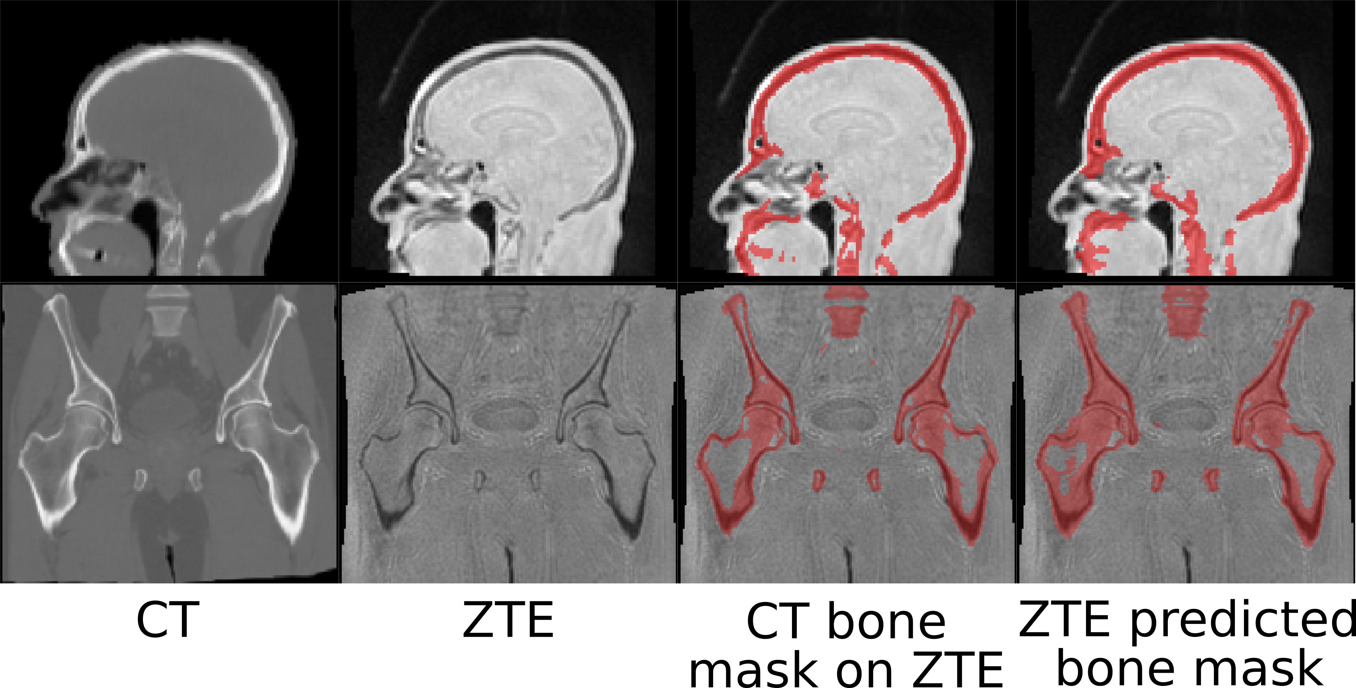
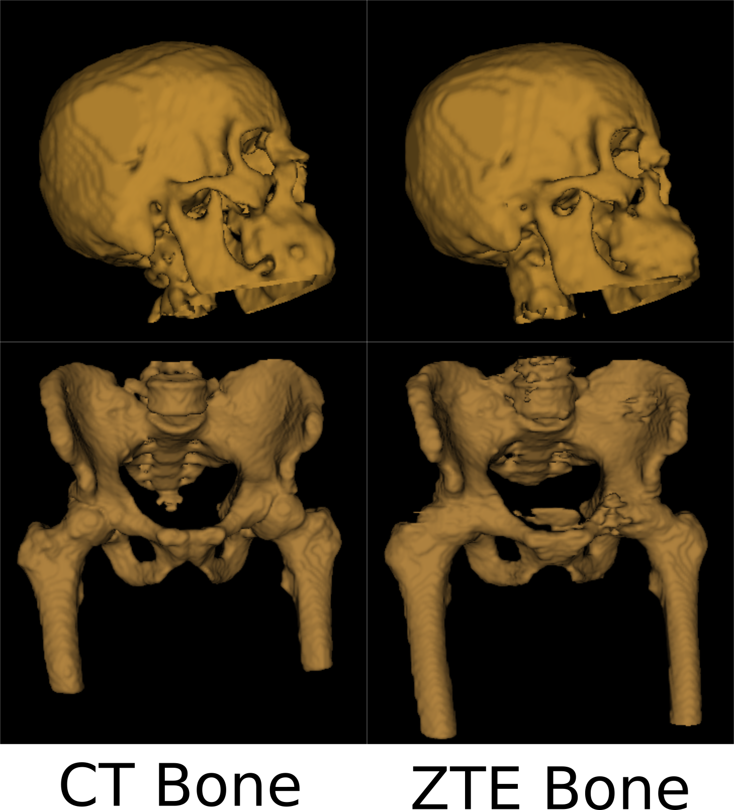
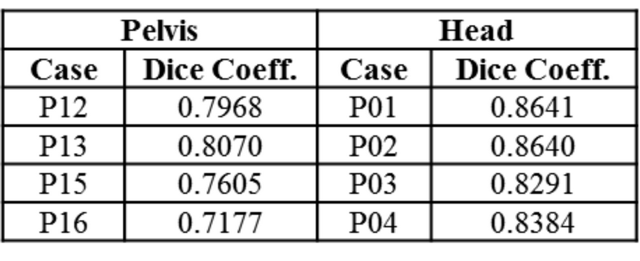
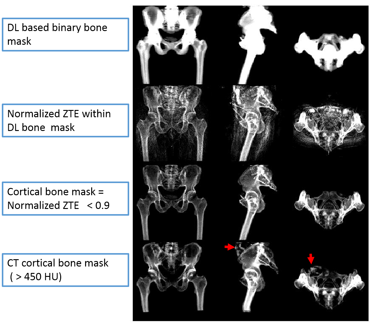
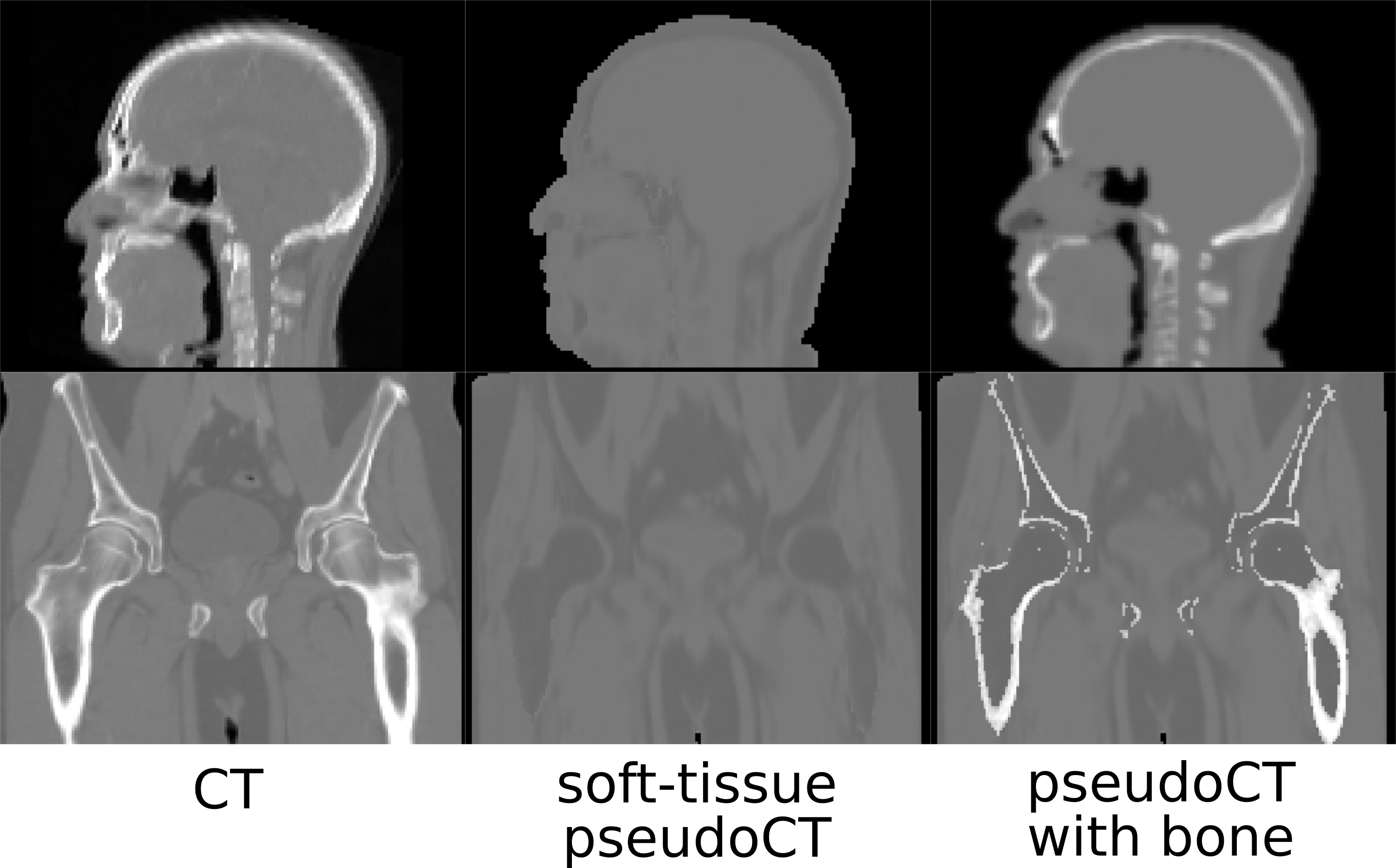
Fig.1 shows typical bone mask images predicted using DL trained model. Qualitative assessment (from Fig.1 and 2) suggests that DL based bone segmentation maintained the shape of bone structures in skull, pelvis, femur, and vertebrae region. Critically, it does not include air-pockets, which is significant since air-pockets have overlapping signal intensity profile with cortical bone. DL bone mask is observed to be slightly over-segmented compared to CT bone (Lower Dice of ~0.71-0.80 (pelvis), and ~0.82-0.86 (head)). However, over-segmentation does not affect pCT fidelity since ZTE data is used for further refinement of bone mask to extract cortical bone (Fig.3). Overall, we notice that cortical bone obtained from DL and ZTE thresholding matches very well to CT cortical bone (Fig.3, pelvis shown). Fig.4 shows that the proposed continuous density pseudoCT generated from Lava-Flex and ZTE matches gold standard CT well.

Conclusion

We have presented a transformation model for generating pCT images from ZTE and Dixon Lava-Flex MR images. We have demonstrated the bone values using model predicted pCT is comparable with bone from true CT image.

Acknowledgements

No acknowledgement found.