0688
Deep learning for fast MR Fingerprinting Reconstruction1Athinoula A. Martinos Center, Charlestown, MA, United States, 2Radiology, Massachusetts General Hospital, Boston, MA, United States, 3Physics, Harvard University, Cambridge, MA, United States
Synopsis
The exponential growth in the number of dictionary entries with increasing dictionary dimensions places a practical limit on the number of tissue parameters that may be simultaneously reconstructed. While a sparse sampling of some dimensions can mitigate the problem it also introduces significant errors into the reconstruction. In this work we demonstrate that Deep Learning methods can be used to train a compact neural network with sparse dictionaries without penalty on the reconstruction accuracy.
Introduction
In MR Fingerprinting (MRF) (1), the evolution of tissue magnetization is used to infer multiple quantitative tissue parameter maps simultaneously by comparison of the acquired signal to a precomputed dictionary of magnetization trajectories. The exponential growth in the number of dictionary entries with increasing dictionary dimensions places a practical limit on the number of tissue parameters that may be simultaneously reconstructed. While a sparse sampling of some dimensions can mitigate the problem it also introduces significant errors into the reconstruction. In this work we demonstrate that Deep Learning (2) methods can be used to train a compact neural network (NN) with sparse dictionaries without penalty on the reconstruction accuracy.Methods
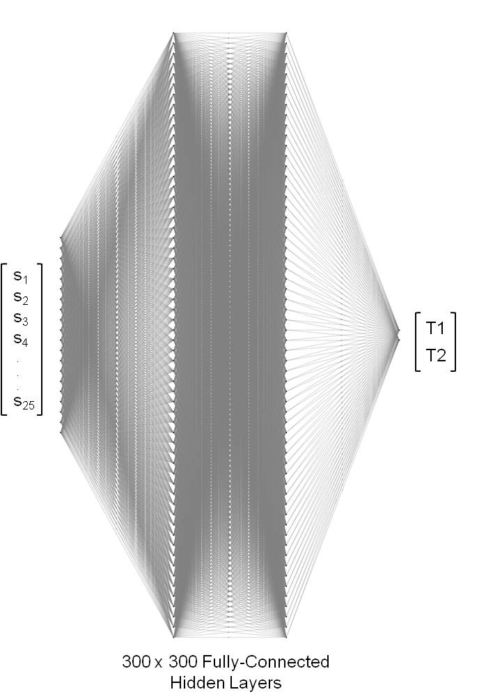
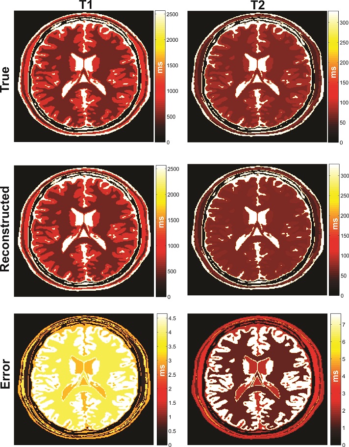
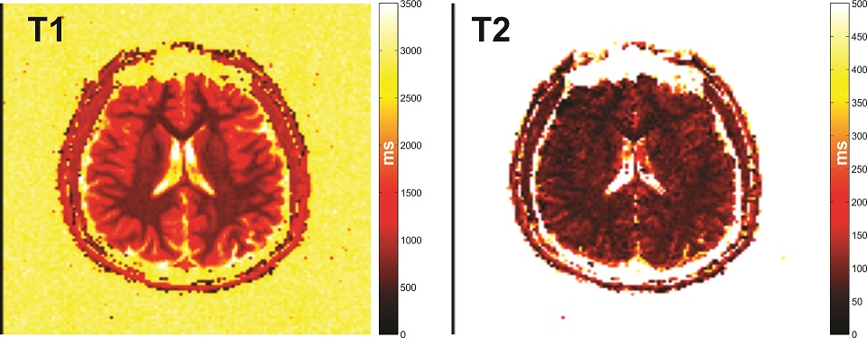
A 25 measurements acquisition schedule was used with our previously described optimized MRF EPI pulse sequence (3–5) to define a training dictionary with 64790 entries composed of T1 values in the range 100-3500 ms and T2 values in the range 1-1100 ms. The total dictionary required 64790×25=1619750 floating-point coefficients for storage. The dictionary was used to train a NN with 300×300 fully connected hidden layers. To test the accuracy of the resulting network, a numerical brain phantom (6) was used to simulate an MRF acquisition using the same acquisition schedule and pulse sequence. The reconstructed T1 and T2 values were compared voxel-wise and the mean error calculated. To test the in vivo applicability of this method, a healthy 31 year old subject was recruited for this study and provided informed IRB-approved consent. The subject was scanned with the MRF EPI sequence on a 1.5T Siemens Avanto scanner (Siemens Healthcare, Erlangen, Germany) using the manufacturer’s body coil for transmit and 32-channel head coil for receive with the following acquisition parameters: TI/TE/BW/Slice Thickness/Resolution/matrix size = 19/27ms/2009 Hz/pixel/5mm/2×2mm2/128×128. An acceleration factor of R=2 was used with the images reconstructed online using the GRAPPA method (7). The acquired data was reconstructed with the presently described NN but with a smaller (6849×25= 171225) training dictionary.Results
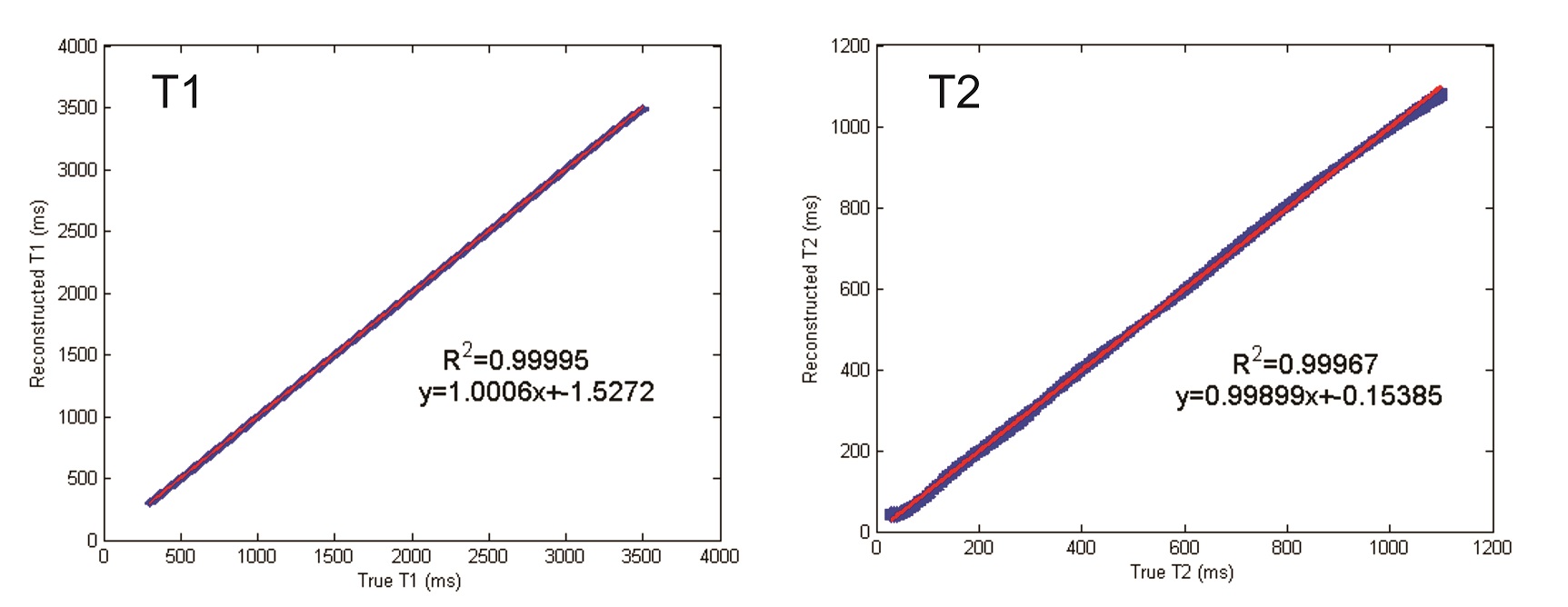
The structure of the resulting NN is shown in Fig. 1 and achieved a twenty-fold compression over the training dictionary requiring only 5% of the floating-point coefficients. The fidelity of the reconstructed training data in comparison to the true values is shown in Fig. 2 for T1 and T2 which both showed excellent agreement to the true values yielding a least-squares correlation coefficient R2 of 0.99/0.99 for T1/T2 and mean±std error in T1/T2 of 3.56±1.17ms/3.54±2.66ms. The true and reconstructed phantom maps are shown in Fig. 3 along with the voxel-wise error map calculated as the absolute difference between the true and reconstructed maps. The reconstructed sample in vivo T1 and T2 maps are shown in Fig. 4.Discussion
Neural networks offer a compressed representation of complex functions that reduces the computational burden in reconstruction of high dimensional data. In contrast to traditional dictionary matching, where the entirety of the dictionary must be stored, once the initial neural network has been trained, only a compact number of coefficients need to be stored for accurate reconstruction. This facilitates wide distribution of the reconstruction network and eliminates the need for large computational resources.Conclusion
We have demonstrated a successful application of MRF reconstruction using Deep Learning techniques. Future work will explore alternative network structures and training datasets to find the optimal configuration.Acknowledgements
No acknowledgement found.References
1. Ma D, Gulani V, Seiberlich N, Liu K, Sunshine JL, Duerk JL, Griswold MA. Magnetic resonance fingerprinting. Nature 2013;495:187–192. doi: 10.1038/nature11971.
2. LeCun Y, Bengio Y, Hinton G. Deep learning. Nature 2015;521:436–444.
3. Cohen O, Sarracanie M, Armstrong BD, Ackerman JL, Rosen MS. Magnetic resonance fingerprinting trajectory optimization. In: Proceedings of the International Society of Magnetic Resonance in Medicine. Milan, Italy; 2014. p. 27.
4. Cohen O, Sarracanie M, Rosen MS, Ackerman JL. In Vivo Optimized MR Fingerprinting in the Human Brain. In: Proceedings of the International Society of Magnetic Resonance in Medicine. Singapore; 2016. p. 430.
5. Cohen O, Armstrong BD, Sarracanie M, Farrar, Christian T., Ackerman Jerome L., Rosen Matthew S. 15T Ultrahigh Field Fast MR Fingerprinting with Optimized Trajectories. In: Proceedings of the International Society of Magnetic Resonance in Medicine. Milan, Italy; 2014. p. 4285.
6. Collins DL, Zijdenbos AP, Kollokian V, Sled JG, Kabani NJ, Holmes CJ, Evans AC. Design and construction of a realistic digital brain phantom. IEEE Trans. Med. Imaging 1998;17:463–468.
7. Griswold MA, Jakob PM, Heidemann RM, Nittka M, Jellus V, Wang J, Kiefer B, Haase A. Generalized autocalibrating partially parallel acquisitions (GRAPPA). Magn. Reson. Med. 2002;47:1202–1210.
Figures