0687

L2 or not L2: Impact of Loss Function Design for Deep Learning MRI Reconstruction

Kerstin Hammernik¹, Florian Knoll^2,3, Daniel K Sodickson^2,3, and Thomas Pock^1,4

¹Institute of Computer Graphics and Vision, Graz University of Technology, Graz, Austria, ²Center for Biomedical Imaging and Center for Advanced Imaging Innovation and Research (CAI2R), NYU School of Medicine, New York, NY, United States, ³Department of Radiology, NYU School of Medicine, New York, NY, United States, ⁴Safety & Security Department, AIT Austrian Institute of Technology GmbH, Vienna, Austria

Synopsis

Human radiologists gain experience from reading numerous MRI images to recognize pathologies and anatomical structures. To integrate this experience into deep learning approaches, two major components are required: We need both a suitable network architecture and a suitable loss function that measures the similarity between the reconstruction and the reference. In this work, we compare pixel-based and patch-based loss functions. We show that it is beneficial to consider other loss functions than the squared L2 norm to get a better representation of the human perceptual system and thus to preserve the texture in the tissue.

Purpose

Deep learning approaches provide a new way to reconstruct MRI images by modeling how human radiologists are usingyears of experience to identify anatomical structures, pathologies, and image artifacts$$$^1$$$. Modeling this experience by deep learning approaches requires not only a suitable network architecture, but also a suitable similarity measure during the training phase. This similarity measure, which is also known as loss function, defines how the reconstruction is compared to the reference image during training. In deep learning approaches, this loss function is often chosen as the squared $$$\mathcal{L}_2$$$ norm, but it has several drawbacks: It compares pixel-wise differences, is not robust against outliers and it represents the human perceptual system poorly$$$^{2,3}$$$. This motivates the use of perceptual-based measures such as Structural Similarity Index (SSIM)$$$^4$$$ that take local patch statistics into account.

Methods

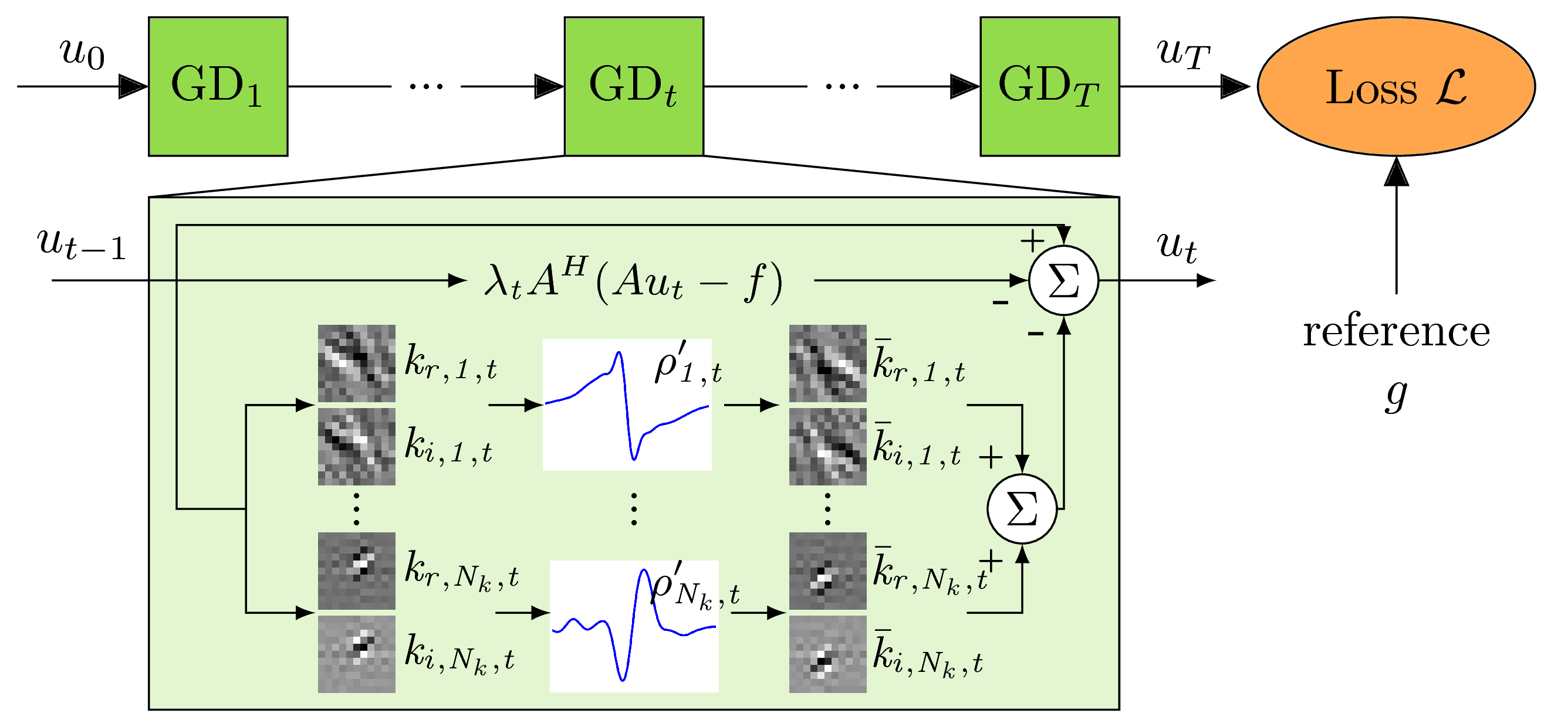
Inspired by deep learning and variational energy minimization, we define a variational network (VN)$$$^1$$$ by an incremental gradient descent (GD) algorithm for $$$T$$$ iterations to obtain a reconstruction $$$u_T\in \mathbb{C}^N$$$:$$u_{t} = u_{t-1} - \alpha_{t-1} \sum\limits_{j=0}^J \nabla h_j(u_{t-1})$$The term $$$\sum\limits_{j=0}^J h_j(u_{t-1})$$$ is defined by the following variational model for MRI reconstruction:$$h_0(u) = \Vert Au - f \Vert_2^2,\quad h_j(u) = \rho_j(k_j*u), j=1...J$$The first term $$$h_0(u)$$$ measures the similarity of the reconstruction $$$u_t$$$ to the acquired k-space data $$$f\in\mathbb{C}^{NQ}$$$ for $$$Q$$$ coils. The forward sampling operator $$$A:\mathbb{C}^{N}\mapsto \mathbb{C}^{QN}$$$ applies the coil-sensitivity profiles, Fourier transforms and the sampling pattern. In the regularization part $$$\sum\limits_{j=1}^J h_j(u)$$$, the complex reconstruction $$$u_t\in \mathbb{C}^N$$$ that can be viewed as a real image with two feature planes $$$u\in\mathbb{R}^{N\times 2}$$$, is convolved with separate filter kernels for the real and imaginary plane $$$k\in\mathbb{R}^{s \times s \times 2}$$$ of size $$$s$$$. The convolution is followed by the application of non-linear functions $$$\rho:\mathbb{R}^{N\times 2}\mapsto\mathbb{R}$$$. Figure 1 illustrates the used VN architecture.

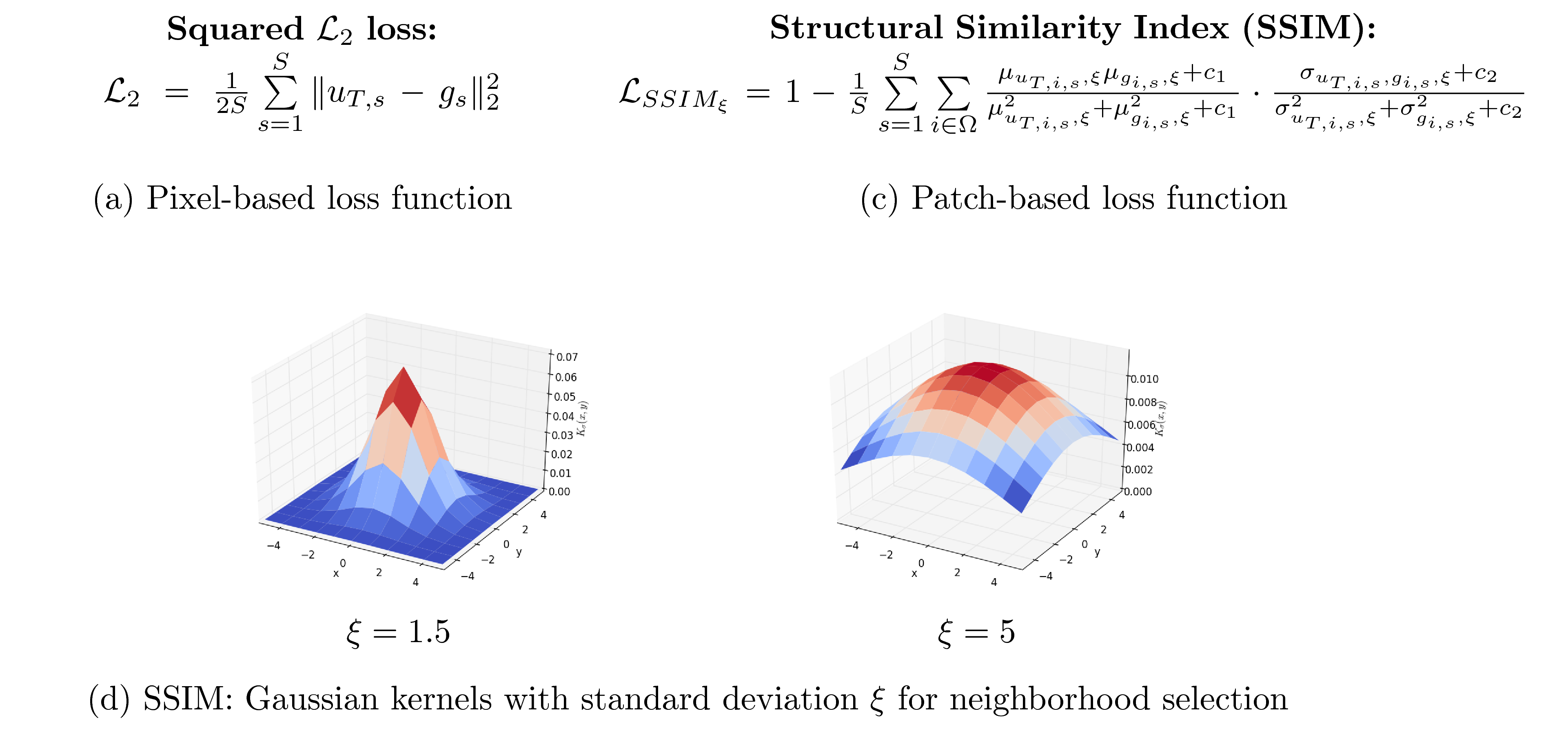
One major key ingredient to train this VN is the loss function which measures the similarity between the reconstruction $$$u_T$$$ and the (fully-sampled) reference $$$g$$$. We train our approach on the pixel-based squared $$$\mathcal{L}_2$$$ loss and the patch-based Structural Similarity Index (SSIM)$$$^3$$$ illustrated in Figure 2. SSIM measures the statistics of a pixel's neighborhood. The extend of the neighborhood is characterized by Gaussian convolution kernels of fixed size and varying standard deviations $$$\xi$$$. The lower $$$\xi$$$ is chosen, the less information about the local statistics can be included in the measure and the more SSIM resembles a pixel-based measure.

Experimental setup

To compare the individual loss functions, we fixed the VN architecture to $$$T=10$$$ steps, and $$$N_k=48$$$ filter kernels of size $$$11\times11$$$ for each step. We evaluated our approach on different sequences of a knee protocol consisting of coronal proton density (corPD), coronal fat-saturated PD (corFS) and axial fat-saturated $$$T_2$$$ (axT2FS) TSE sequences. For each sequence, we scanned 10 patients on a clinical 3T system (Siemens Magnetom Skyra) using a 15-channel knee coil. The study was approved by the IRB. The sequence parameters were TR=2800ms, TE=27ms, turbo factor TF=4, matrix size 320x288 for corPD, TR=2870ms, TE=33, TF=4, matrix size 320x288 for corFS and TR=4000ms, TE=65ms, TF=4, matrix size 320x256 for axT2FS. Coil sensitivity maps were precomputed using ESPIRIT$$$^5$$$. We trained individual networks for each loss function on all contrasts for acceleration factor $$$R\in\{3,4\}$$$ using 5 patients and 20 slices from each patient. For the SSIM loss, we use Gaussian convolution kernels with standard deviations $$$\xi\in\{1.5,5\}$$$.

Results

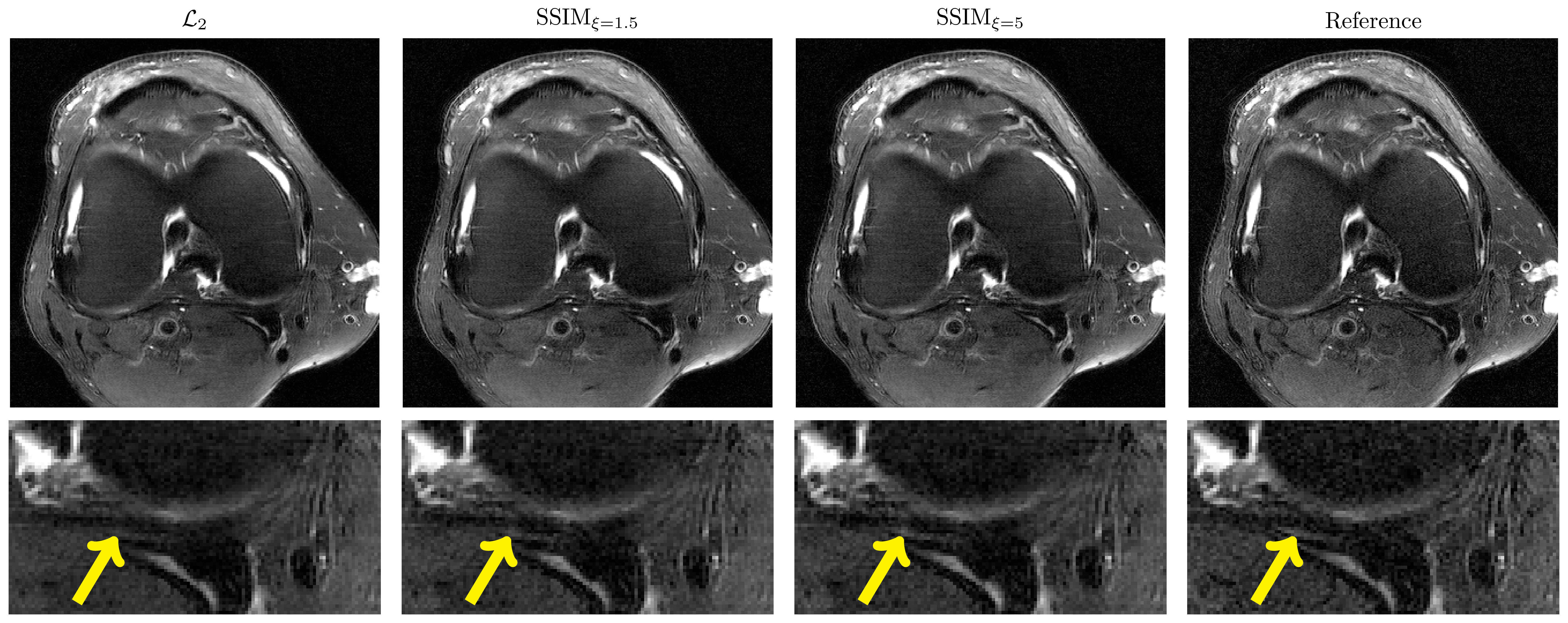
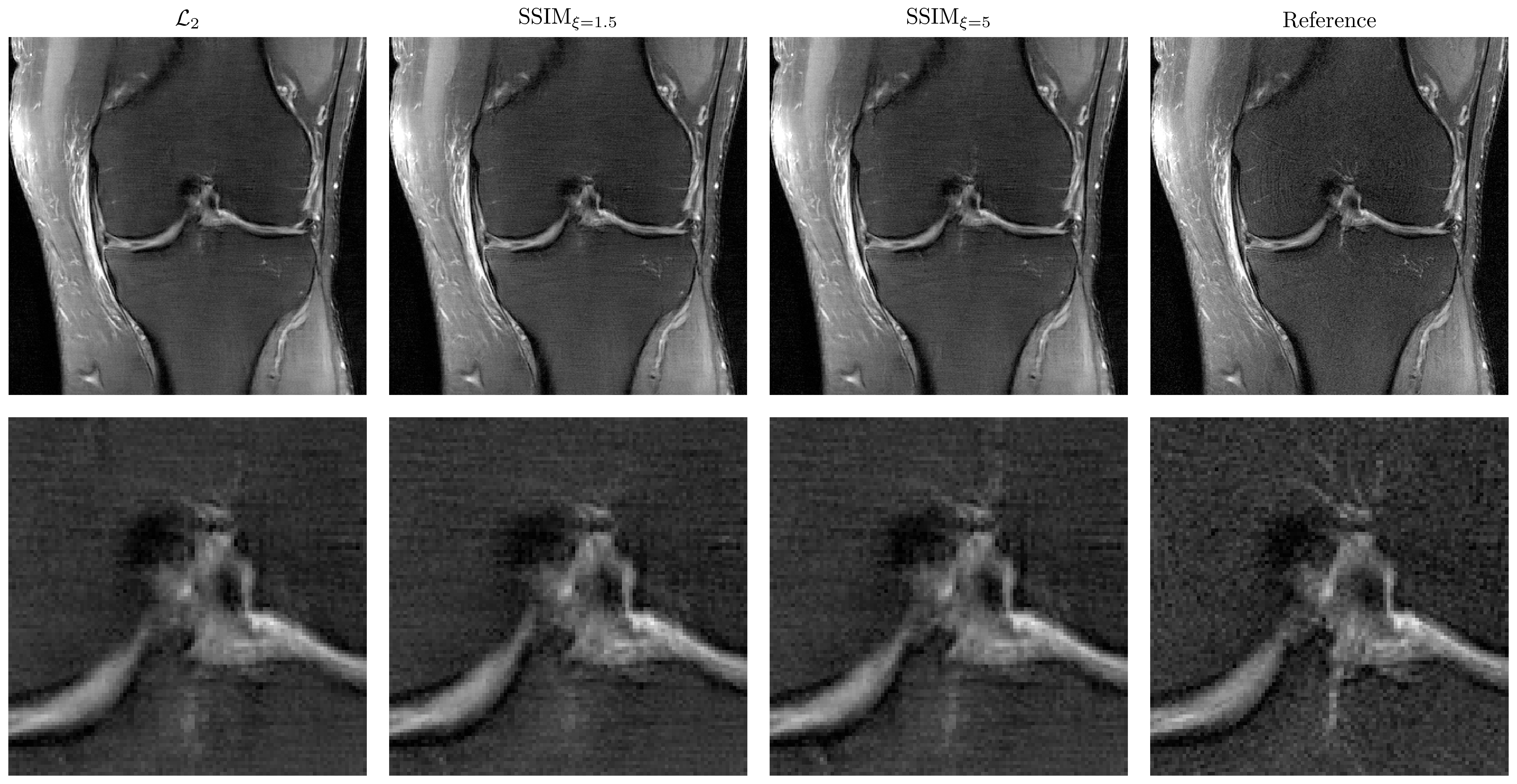
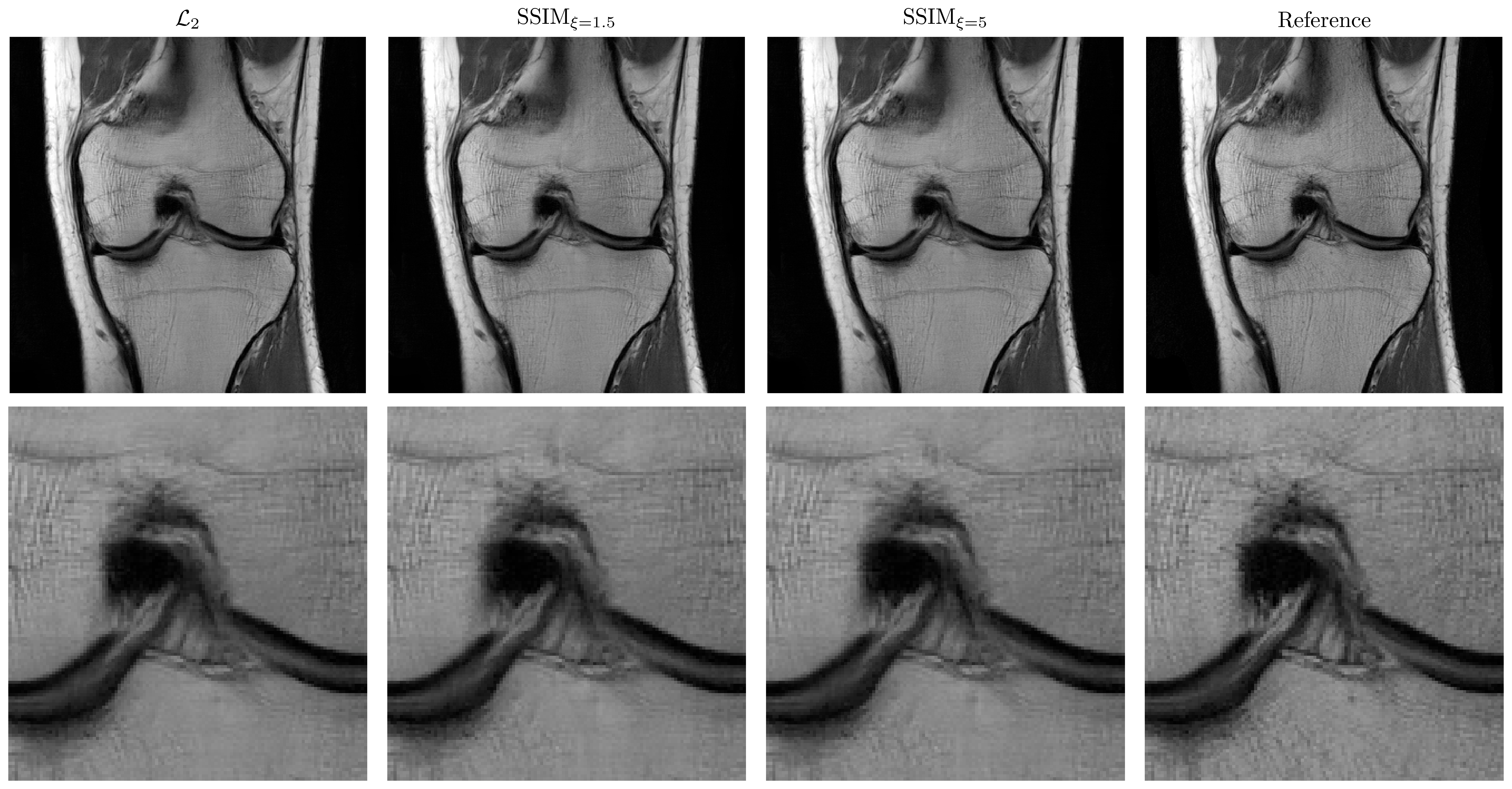
Figure 3 illustrates the results for the axT2FS sequence for $$$R=3$$$. For acceleration factor $$$R=4$$$, results for corFS and corPD are depicted in Figure 4 and Figure 5. All results illustrate similar behavior: The SSIM results show improved sharpness, details and texture of the reconstructions compared to $$$\mathcal{L}_2$$$. This effect is stronger when increasing the pixel coverage $$$\xi$$$ to 5.

Discussion

This work compares pixel-based and patch-based loss functions for a deep learning approach. Our results show that using SSIM as loss function, which provides a better description of the human perception system during training, results in sharper images compared to the pixel-based $$$\mathcal{L}_2$$$ loss. Future work will include investigations of more sophisticated loss functions that combine the advantages of both pixel-based and patch-based approaches or multi-scale approaches such as MS-SSIM$$$^6$$$.

Acknowledgements

We acknowledge grant support from the Austrian Science Fund (FWF) under the START project BIVISION, No. Y729, NIH P41 EB017183, NIH R01 EB000447 and NVIDIA corporation.

References

1. K. Hammernik, F. Knoll, D. K. Sodickson, and T. Pock, “Learning a Variational Model for Compressed Sensing MRI Reconstruction”, Proceedings of the International Society of Magnetic Resonance in Medicine (ISMRM), no. 24, p. 1088, 2016.

2. Z. Wang and A. C. Bovik, “Mean squared error: Love it or leave it? A new look at Signal Fidelity Measures”, IEEE Signal Processing Magazine, vol. 26, no. 1, 2009.

3. H. Zhao, O. Gallo, I. Frosio, and J. Kautz, “Loss Functions for Neural Networks for Image Processing”, arXiv:1511.08861, 2015.

4. Z. Wang, A. C. Bovik, H. R. Sheikh, E. P. Simoncelli, “Image quality assessment: from error visibility to structural similarity”, IEEE Transactions on Image Processing, vol. 13, no. 4, pp. 600–612, 2004.

5. M. Uecker, P. Lai, M. J. Murphy, et al., “ESPIRiT-an eigenvalue approach to autocalibrating parallel MRI: where SENSE meets GRAPPA”, Magn Reson Med, vol. 71, no. 3, pp.990–1001, 2014.

6. Z. Wang, E. P. Simoncelli and A. C. Bovik, “Multi-scale structural similarity for image quality assessment”, IEEE Asilomar Conference on Signals, Systems and Computers, vol. 2, pp. 1398–1402, 2003.

Figures

Figure 1: Our variational network (VN) architecture consists of $$$T$$$ incremental gradient descent (GD) steps, where each step implements the depicted scheme. As the image $$$u_t$$$ is complex, we learn separate filter kernels $$$k$$$ for the real $$$r$$$ and complex plane $$$i$$$. The activation function $$$\rho': \mathbb{R}^{N\times 2}\mapsto\mathbb{R}^N$$$ combines the information of the two feature planes. During training, we compare the similarity between the VN output $$$u_T$$$ with a reference $$$g$$$ using a loss function. The gradient information of the loss $$$\mathcal{L}$$$ is used to update the parameters (kernels $$$k$$$, regularization parameter $$$\lambda$$$ and activation functions $$$\rho'$$$) during training.

Figure 2: We use the pixel-based $$$\mathcal{L}_2$$$ loss function (a) where $$$u_T$$$ denotes the reconstruction, $$$g$$$ is the reference and $$$S$$$ is the number of training samples. In contrast, perceptual-based loss functions such as SSIM (c) estimate the value around a certain neighborhood. This neighborhood is defined by a Gaussian window $$$\xi$$$ for SSIM, controlling the pixel-coverage as illustrated in (d). The SSIM value is estimated using patch means $$$\mu_{u_{i,s},\xi},\,\mu_{g_{i,s},\xi}$$$ , variances $$$\sigma_{u_{i,s},\xi}^2,\,\sigma_{g_{i,s},\xi}^2$$$ and covariance $$$\sigma_{u_{i,s},g_{i,s},\xi}$$$ and depends on user-defined constants $$$c_1,\,c_2$$$.

Figure 3: Comparison of network results trained with different loss functions for axT2FS $$$R=3$$$. The results for the network that was trained with SSIM appear slightly sharper with increasing standard deviation $$$\xi$$$ of the used Gaussian window kernel compared to $$$\mathcal{L}_2$$$. This can be especially seen on the structure highlighted by the yellow arrow.

Figure 4: Comparison of network results trained with different loss functions for corPDFS $$$R=4$$$. The results for the patch-based approach SSIM appear slightly sharper than the result for the pixel-based $$$\mathcal{L}_2$$$ loss.

Figure 5: Comparison of network results trained with different loss functions for corPD $$$R=4$$$. The results for the patch-based approach SSIM appear slightly sharper than the result for the pixel-based $$$\mathcal{L}_2$$$ loss.

Proc. Intl. Soc. Mag. Reson. Med. 25 (2017)

0687