0643
A Deep Cascade of Convolutional Neural Networks for MR Image Reconstruction1Department of Computing, Imperial College London, London, United Kingdom, 2King's College London, 3Imperial College London
Synopsis
The acquisition of Magnetic Resonance Imaging (MRI) is inherently slow. Inspired by recent advances in deep learning, we propose a framework for reconstructing MRI images from undersampled data using a deep cascade of convolutional neural networks. We show, for Cartesian undersampling of 2D cardiac MR images, the proposed deep learning reconstruction method outperforms the state-of-the-art compressed sensing approaches, such as dictionary learning-based MRI (DLMRI) reconstruction, both in terms of reconstruction error, the perceptual quality and the reconstruction speed for 4-fold and 8-fold undersampling.
Purpose
The aim of this study is to accelerate the MRI data acquisition, to reduce the demands on patients, by reducing the amount of k-space data needed for reconstructing images from undersampled data. We aim to evaluate the applicability of deep learning techniques to the MRI reconstruction problem. Deep learning methods have become the state-of-the-art for many imaging problems in computer vision, however, they have not been extensively applied for medical image reconstruction.Method
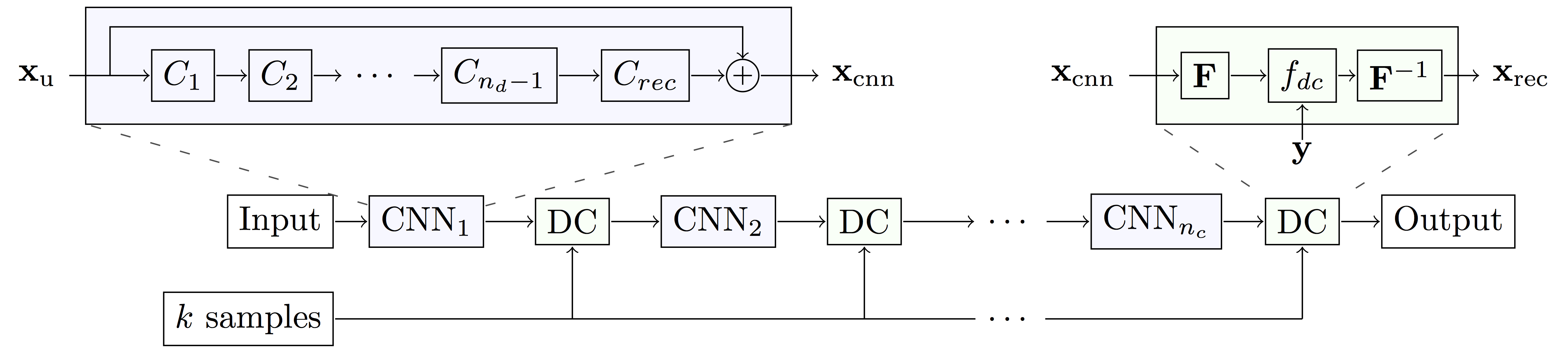
A convolutional neural network (CNN) is a model composed of multiple layers of learnable filters, which can be trained to extract discriminative features of the input useful for producing a desired output, such as image labels and segmentation maps. We hypothesise that CNNs can also be trained to exploit data redundancy through learned representations and hence reconstruct the undersampled images. In our case, the CNN takes in an undersampled image and directly produces the reconstruction.
To further improve the quality of reconstruction produced by CNN, we introduce a data consistency layer (DC), which ensures the data fidelity of the intermediate reconstruction. The DC layer replaces the k-space values of the CNN reconstruction with the acquired data, but only if the entry has been sampled originally. To map the images between the image domain and k-space, Discrete Fourier Transform is used.
We form a cascade of CNNs by interleaving the DC layer in between multiple instances of CNNs. The architecture of each CNN is inspired by state-of-the-art results in the field.1,2 Our final architecture is 30-layers deep as illustrated in Figure 1: we used 5 CNN’s of which each has 5 convolution filters, interleaved by 5 DC layers.
Experiment: We trained our CNN using fully sampled, short-axis cardiac cine MR scans from 10 volunteers.3 Each scan contains a single slice SSFP acquisition with 30 temporal frames, resolution of 256x256 pixels, FOV of 320x320 mm with slice thickness 10mm. The images were retrospectively undersampled respecting a linear frequency/phase encode structure, while the central 8 lines in k-space were always included.
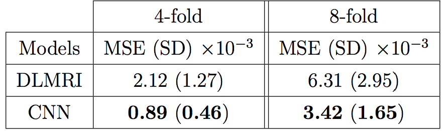
The method was compared to DLMRI4, a state-of-the-art compressed sensing (CS) approach, using the above dataset with undersampling rate of 4-fold and 8-fold. We performed 2-fold cross validation to aggregate the mean and the standard deviation of pixel-wise mean squared error for all individual images. To test our hypothesis that the CNN approach achieves lower error, we used one-sided, paired Wilcoxon signed-rank test. We also compared their perceptual quality and the reconstruction speed.
Results
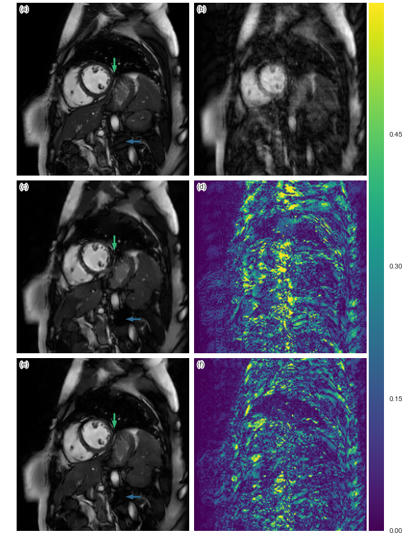
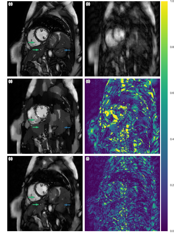
The quantitative result is summarized in Figure 2. The proposed method has lower reconstruction error for both 4x and 8x undersampling. Indeed, the Wilcoxon test yields great statistical significance (p << 0.001). Examples of reconstructions are shown in Figure 3 (4x undersampling) and Figure 4 (8x undersampling). For high undersampling rates, DLMRI generated block-like artefacts. In contrast, with CNN-based reconstruction, even though it also suffered from blurring out some of the components, it managed to generate more homogeneous images, at the same time recovering most anatomical structures more accurately. To reconstruct the full volume for each scan, DLMRI took 6.1±1.3 hours on a CPU. While training the CNN took approximately 3 days on GeForce GTX 1080, the reconstruction only took 23±0.1ms per timeframe.Discussion and Conclusion
While CS-based methods provide a mathematically rigorous specification for robust signal recovery, when the number of samples acquired is not sufficient, their reconstructions are not necessarily perceptually appealing. In contrast, we have empirically shown that CNN-based approaches can reconstruct images better than DLMRI for 4x and 8x undersampling. CNN modelling outperforms dictionary learning because it can directly model non-linear transformations and learn optimal features of data without specifying hard-constraints such as sparsity. While both DLMRI and CNN-based reconstruction suffered from the loss of some anatomical details, the latter is still useful if only near perfect reconstruction is needed for the subsequent analysis, such as tissue segmentation. Another advantage of CNN is that the images can be reconstructed extremely fast, potentially offering real-time applications.
For this work, we restricted our considerations for 2D static image reconstruction from Cartesian undersampling. In practice most MRI scanners implement advanced acquisition protocols, such as parallel acquisition or interpolating dynamic sequences. Our approach must be adapted to these, however, it is expected that the method will perform better, as the redundancy in their respective methods can also be exploited for the CNN reconstructions. Although CNNs can only learn local representations which should not affect global structure, it remains to be determined how the CNN approach operates when there is pathology or other more variable content.
Acknowledgements
The research was funded by The Engineering and Physical Sciences Research Council (EPSRC).References
1. Kaiming He et al., “Deep Residual Learning for Image Recognition,” Arxiv.Org, 7(3):171–180, 2015.
2. Karen Simonyan et al., “Very deep convolutional networks for large-scale image recognition,” ICLR, pages 1–14, 2015.
3. J. Caballero et al., “Dictionary Learning and Time Sparsity for Dynamic MR Data Reconstruction,” IEEE Transactions on Medical Imaging, vol. 33, no. 4, pp. 979–994, 2014.
4. S. Ravishankar et al., “MR Image Reconstruction From Highly Undersampled k-Space Data by Dictionary Learning,” IEEE Transactions on Medical Imaging, vol. 30, pp. 1028–1041, May 2011.
Figures