0641
Compressed sensing and Parallel MRI using deep residual learning1Korea Advanced Institute of Science and Technology, Daejeon, Korea, Republic of
Synopsis
A deep residual learning algorithm is proposed to reconstruct MR images from highly down-sampled k-space data. After formulating a compressed sensing problem as a residual regression problem, a deep convolutional neural network (CNN) was designed to learn the aliasing artifacts. The residual learning algorithm took only 30-40ms with significantly better reconstruction performance compared to GRAPPA and the state-of-the-art compressed sensing algorithm, ALOHA.
Introduction
Compressed sensing (CS) is one of powerful ways to reduce the scan time of MR imaging with performance guarantee. However, computational cost of CS is usually expensive. To solve this problem, we propose a novel deep residual learning algorithm to reconstruct MR images from highly down-sampled k-space data. Based on the observation that the coherent aliasing artifacts from down-sampled data have topologically simpler structure than the original image data, we formulate a CS problem as a residual regression problem and proposed a deep convolutional neural network (CNN) to learn the aliasing artifacts.
Theory
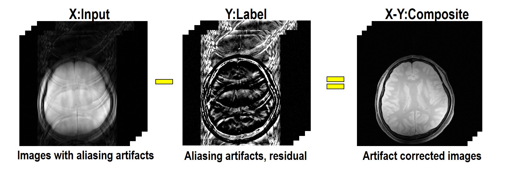
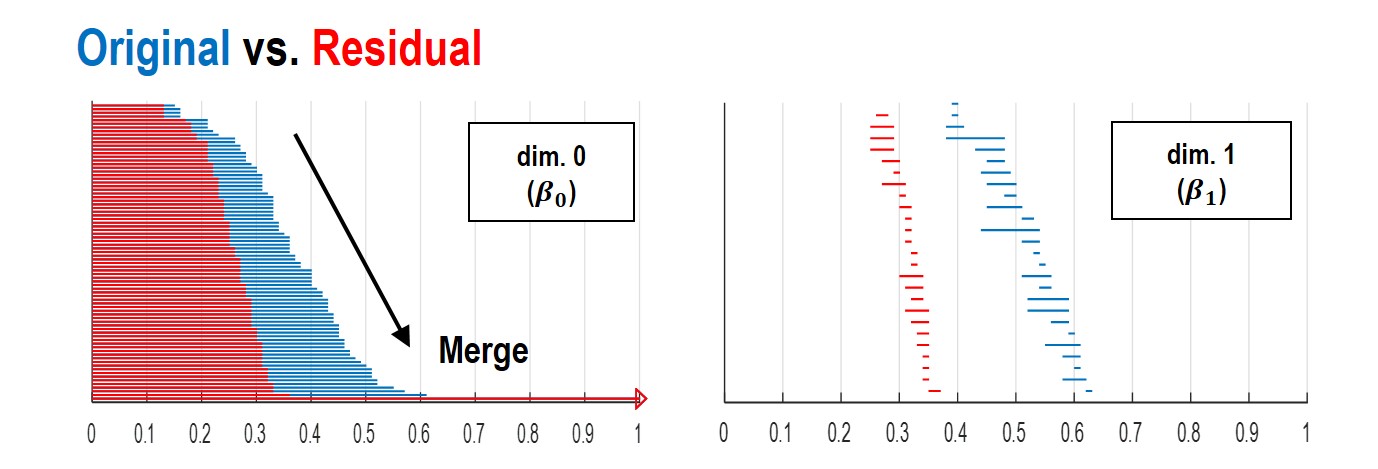
As shown in Fig.1, our main idea is to estimate the label $$$Y$$$ composed of residual (aliasing artifacts) from down-sampled reconstruction input ($$$X$$$). After the aliasing artifacts are estimated, we could obtain an aliasing-free image by subtracting the estimated aliasing artifact from the aliased inputs ($$$X-Y$$$). This network architecture is proposed based on our conjecture that aliasing artifacts from uniformly under-sampled patterns have simpler topological structure. According to the statistical learning theory[1], the risk of a learning algorithm is bounded in terms of a complexity measure and the empirical risk. Thus, for a given network architecture, if the manifold of label $$$Y$$$ is simple, then the risk can be reduced and the performance of the learning algorithm can be improved. To prove our conjecture, we employed the recent topology tool called persistent homology[2] to investigate the topological structure of aliasing artifact and the original images, respectively. As shown in Fig.2, Betti numbers ($$$\beta_0,\beta_1$$$) decayed much more quickly in the residual learning, implying that the residual image space has simpler topology than the original one. Based on this, we implemented a deep residual learning architecture.Materials & Methods
By utilizing the convolution, batch normalization, rectified linear unit (ReLU) and contracting path connection with concatenation[3,4], we employed residual learning network[3] using U-net[4] structure which has additional pooling and unpooling layers (convolution transpose) on the deconvolution network framework[5] (See Fig.3).
Total 81 axial brain MR images from 9 subjects (3T Siemens, Verio) were used for our experiments. Here are the scan parameters for SE and GRE scans; TR 3000-4000ms, 256$$$\times$$$256 matrix, 5mm slice thickness, TE 4-20ms, 4 coils, FOV 240$$$\times$$$240, FA 90 degrees. For the dataset, we split the training and test data set by randomly choosing about 80% of total images for training and about 20% for testing. Also, we generated 32 times more training samples by rotation, shearing and flipping for data augmentation. For single-channel experiments, we chose 1 channel data from the four channel data.
The original k-spaces were 4 times down-sampled retrospectively with 13 ACS lines (5% of total PE). The residual images are constructed by the difference between the fully sampled data and the down-sampled data (Fig.1). The residual images were used as labels $$$Y$$$ and the images from down-sampled data were used as input $$$X$$$. We trained the network using the magnitude of MR images by stochastic gradient descent method with momentum. Followings are H/W and S/W environment specification; GPU GTX 1080, CPU i7-4770 (3.40GHz), MatConvNet toolbox (ver.20, http://www.vlfeat.org/matconvnet/) in MATLAB 2015a (Mathworks, Natick). The reconstruction results of GRAPPA and ALOHA[6] were also presented to compare and verify the performance of the proposed network.
Result & Discussion
The reconstruction results of single channel experiment are shown in Fig.4(b). In the zero-filled reconstruction image, there is significant amount of aliasing artifacts. Moreover, due to coherent aliasing artifacts from uniform down-sampling, most of the existing CS algorithm failed, and only ALOHA was somewhat successful with slight remaining aliasing artifact. However, the result of residual learning produced almost perfect reconstruction results by removing the coherent aliasing artifacts. In four-channel experiments in Fig.4(c), GRAPPA shows the strong aliasing artifacts due to the insufficient number of coils and ACS lines. ALOHA reconstruction could remove most of the aliasing artifacts, but still remains slight artifacts due to the coherent sampling. However, the proposed method provided near perfect reconstruction result visually and quantitatively.
The training of the proposed network took 9 hours. However, it only takes 30ms and 41ms to reconstruct single-channel and multi-channel data, respectively. The reconstruction time of GRAPPA is 30sec and that of ALOHA were about 2min and 10min for single-channel and multi-channel data, respectively.
Conclusion
In this study, we proposed a reconstruction method for accelerated MRI from uniform down-sampled MR brain data via deep residual learning. The proposed network produces accurate results instantly compared to many existing CS algorithms which require heavy computational costs.Acknowledgements
This study was supported by Korea Science and Engineering Foundation under Grant NRF-2016R1A2B3008104.References
[1] Martin A et al. Neural network learning: Theoretical foundations. Cambridge Univ. Press, 2009.
[2] Edelsbrunner H et al. Persistent homology-a survey, Contemporary Mathematics, 2008;453:257-282
[3] He K et al. Deep residual learning for image recognition, CVPR, 2016.
[4] Ronneberger O et al. U-net: Convolutional networks for biomedical image segmentation, MICCAI, 2015;234-241
[5] Noh H, et al. Learning deconvolution network for semantic segmentation, Proc. of IEEE ICCV, 2015;1520-1528
[6] Jin KH et al. A general framework for compressed sensing and parallel MRI using annihilating filter based low-rank Hankel matrix, IEEE Trans. Computational Imaging, 2016;2(4):480-495
Figures