0622
Evaluation of Approximation Method for B1+ Correction using Digital Reference Object in Prostate DCE-MRI1Department of Radiological Sciences, University of California, Los Angeles, Los Angeles, CA, United States, 2Physics and Biology in Medicine IDP, University of California, Los Angeles, Los Angeles, CA, United States, 3Department of Electrical Engineering, University of Southern California, Los Angeles, CA, United States
Synopsis
A digital reference object (DRO) for prostate dynamic contrast-enhanced MRI application is created by modifying DRO created by the
Purpose
Quantitative dynamic contrast-enhanced MRI (DCE-MRI) has shown great potential to improve the detection and grading of prostatic carcinoma (PCa).1 However, DCE-MRI pharmacokinetic (PK) modeling1 is sensitive to B1+ inhomogeneity, compromising absolute quantitation on 3.0T systems2. B1+ variation is on the order of 10-15% in the prostate at 3.0T3. Correction of B1+ variation is critical to improving the DCE-MRI quantification, but to date, adoption of B1+ correction has been limited due to its required integration with PK modeling. We recently proposed a practical method to correct B1+ variation4 (Figure 1), and in this work, we evaluate its efficacy using a digital reference object (DRO), modified from the DRO of the RSNA Quantitative Imaging Biomarkers Alliance (QIBA)5. Practical considerations, such as fitting method, arterial input function (AIF) selection, and noise level, were included.Methods
Assumed standard Tofts model6 and a population-averaged AIF, the B1+ correction can be simplified according to Taylor series approximations under certain conditions: i) small flip angle (FA), ii) small $$$\frac{TR}{T_{10}}$$$,and iii) k ≈ 1, where T10 is pre-contrast T1 and k reflects relative B1 variation, calculated by $$$\frac{FA'}{FA}$$$. Provided these conditions are satisfied, we can express the B1+ correction process as i) Ktrans'/Ktrans ≈ k2, ii) ve'/ve ≈ k2, and iii) kep'/kep ≈ 1, where FA, Ktrans, ve and kep are original values and FA’, Ktrans’, ve’ and kep’ are B1+ corrected values. Note that the proposed model now becomes independent of T10, Ktrans, ve, and kep, enabling the direct B1+ correction of PK parameters without reinitiating pixel-by-pixel PK analysis, as described in Figure 1.
For evaluation of the approximation approach, we utilized the modified QIBA DRO, which are synthetic images derived from mathematical models designed for PK-modeling evaluation. By recreating the DRO according to the description,5 we confirmed our in-house DCE-MRI analysis software. One representative point signal comparison is shown in Figure 2. The imaging protocol was then adjusted according to our prostate DCE-MRI protocol: flip angles (FAs) for T10 mapping = 2°, 5°, 10°, and 15°, dynamic acquisition FA = 12°, TR = 4ms. Ktrans ranges [0.01, 0.02, 0.05, 0.1, 0.2, 0.35] min-1 and ve ranges [0.01, 0.05, 0.1, 0.2, 0.5] as designed for QIBA DRO. As shown in Figure 3, each 2×2 pixel patch contains one specific Ktrans and ve combination.
To account for practical issues, we included three considerations in the evaluation: i) Levenberg-Marquardt (Lev-Mar) algorithms with and without a boundary condition (upper bound for ve to be 1.0), ii) three commonly used population-based AIFs, including Parker7, Weinmann8, and Fritz-Hans9, and iii) two noise levels added following equation $$$A = \sqrt{(R+r_1)^2+r_2^2}$$$ , where R is the original signal, r1 and r2 are noise with mean of 0 and standard deviation of σ, similar to QIBA DRO v9. σ is chosen as 1, 5 and 10, respectively.
Results and Discussion
All results are based on B1+ of 20%, which could introduce around 40% error in PK estimation. We have shown that the error of approximation correction increases with B1+ increases in previous work, so for B1+ range in the prostate application(10-15%), the error should be even smaller than those shown here. The correction errors, computed by percentage error compared to the ground truth (Figure 3). Figure 4 shows Ktrans and ve error comparison between bounded and non-bounded fitting for three AIF inputs. The approximation method performs slightly better in the non-bounded fitting (maximum error<0.23%) as expected. In the bounded fitting, the performance of approximation correction with low ve and high Ktrans combinations are not as good, but the errors are still small (maximum error < 1.48 %). When adding noise with σ of 5 to DRO signal, figure 5 shows that the approximation correction gives almost the same estimation as the conventional correction.Conclusion
We have demonstrated the efficacy of an approximate B1+ correction method for DCE-MRI, using a prostate DRO and a broad range of fitting methods, AIFs, and realistic noise levels. PK modeling error introduced by the approximation method is negligible (error < 1.48%) and the approximation correction did not introduce additional error in the presence of realistic noise, suggesting this as a practical solution for the B1+ correction in prostate DCE-MRI at 3T.Acknowledgements
No acknowledgement found.References
[1] Franiel T, Hamm B, Hricak H. Dynamic contrast-enhanced magnetic resonance imaging and pharmacokinetic models in prostate cancer. Eur Radiol. 2011;21:616-626. doi:10.1007/s00330-010-2037-7
[2] Azlan C a., Di Giovanni P, Ahearn TS, Semple SIK, Gilbert FJ, Redpath TW. B1 transmission-field inhomogeneity and enhancement ratio errors in dynamic contrast-enhanced MRI (DCE-MRI) of the breast at 3T. J Magn Reson Imaging. 2010;31:234-239. doi:10.1002/jmri.22018.
[3] Xinran Z, et al, Clinical Assessment of B1+ Inhomogeneity Effects on Quantitative Prostate MRI at 3.0 T, ISMRM, 2015 #1159
[4] Xinran Z, et al, B1+ Inhomogeneity Correction for Estimation of Pharmacokinetic Parameters through an Approximation Approach, ISMRM, 2016 #2491
[5] Daniel PB et al. https://sites.duke.edu/dblab/qibacontent
[6] Tofts PS. Modeling tracer kinetics in dynamic Gd-DTPA MR imaging. J Magn Reson Imaging. 1997;7(1):91-101. doi:10.1002/jmri.1880070113.
[7] Parker GJM, Roberts C, Macdonald A, et al. Experimentally-derived functional form for a population-averaged high-temporal-resolution arterial input function for dynamic contrast-enhanced MRI. Magn Reson Med. 2006;56(October 2005):993-1000. doi:10.1002/mrm.21066.
[8] Weinmann HJ, Laniado M, Mützel W. Pharmacokinetics of GdDTPA/dimeglumine after intravenous injection into healthy volunteers. Physiol Chem Phys Med NMR. 1984;16(2):167-172. http://www.ncbi.nlm.nih.gov/pubmed/6505043.
[9] Fritz-Hansen T, Rostrup E, Larsson HB, Søndergaard L, Ring P, Henriksen O. Measurement of the arterial concentration of Gd-DTPA using MRI: a step toward quantitative perfusion imaging. Magn Reson Med. 1996;36(2):225-231. doi:10.1002/mrm.1910360209.
Figures
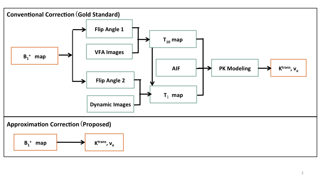
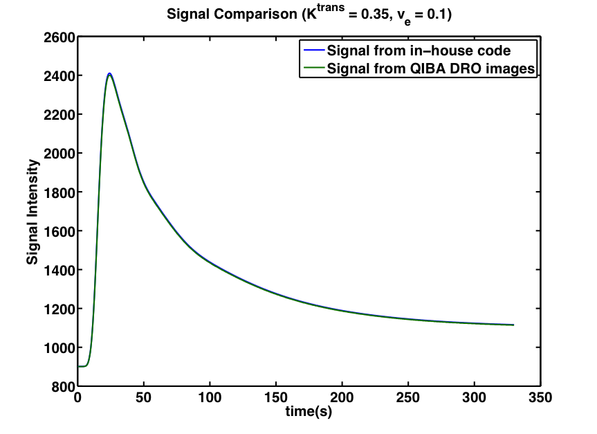
Figure 2. Comparison between Signal from our in-house code and signal from QIBA DRO in one representative point (Ktrans = 0.35 min-1 and ve = 0.1) to confirm our implementation.
After confirmation of our code and model, we could modify the DRO for our prostate cancer application.
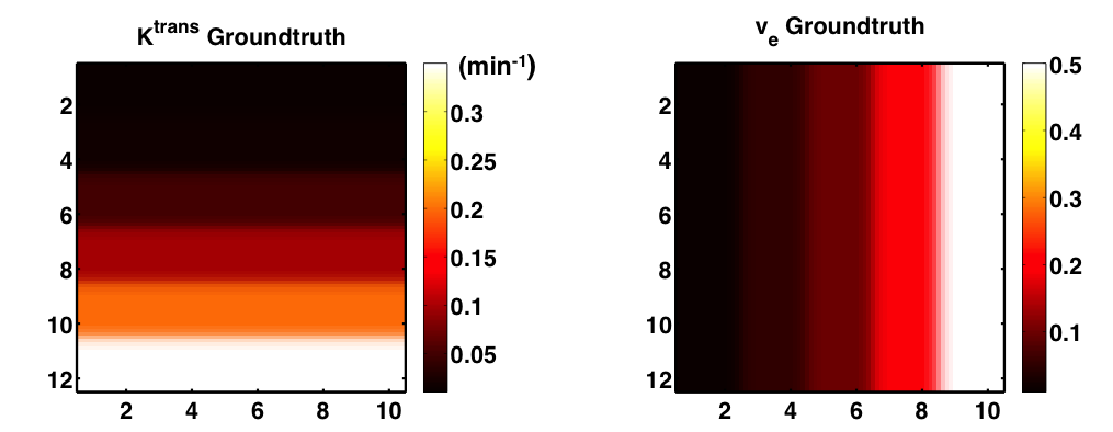
Figure 3. PK parameters assumed in our DRO, which is used as ground truth to evaluate correction methods. Ktrans range: [0.01, 0.02, 0.05, 0.1, 0.2, 0.35] min-1, ve range: [0.01, 0.05, 0.1, 0.2, 0.5]
Each 2×2 pixel patch contains one specific Ktrans and ve combination.
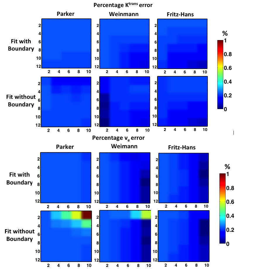
Figure 4. Percentage error of Ktrans and ve from approximation correction method for both fitting setups and for three AIFs.
Comparing the results among different AIFs and fitting methods, the approximation introduced errors are consistent and small.
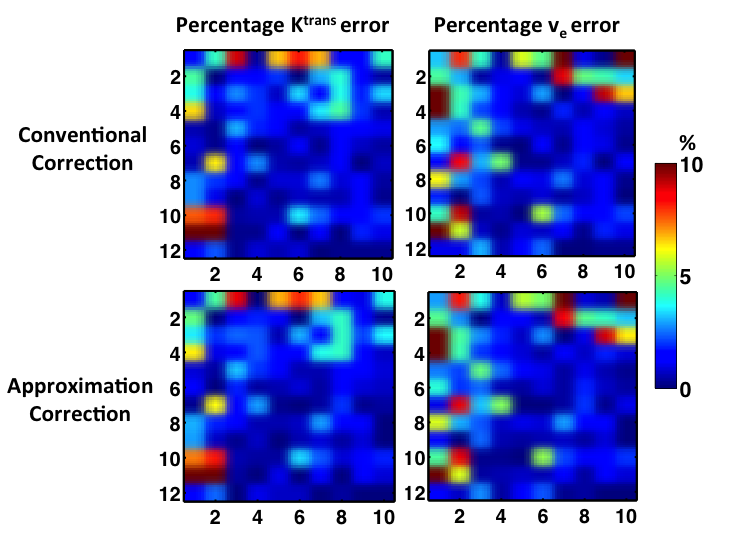
Figure 5. Percentage Ktrans and ve error introduced to both conventional correction method (top row) and approximation correction method (bottom row) by adding noise with σ of 5.
The approximation correction gives almost the same estimation as the conventional method.