0580
3D-EPI-CAIPI and 2D-Multiband-EPI: which is best for fMRI at 3T?1Wellcome Trust Centre for Neuroimaging, UCL Institute of Neurology, London, United Kingdom
Synopsis
2D-MB-EPI and 3D-EPI-CAIPI acquisition schemes can be used to increase spatiotemporal resolution in fMRI. This study examined which approach is optimal at 3T, over a range of temporal and spatial resolutions, while maintaining extended brain coverage. 10 protocols were tested in vivo for each sequence spanning low and high spatial resolution and a range of through-plane acceleration factors. 3D-EPI-CAIPI outperforms 2D-MB-EPI at lower temporal resolutions, as long as physiological effects are corrected and the maximal CAIPIRINHA shift is used. The benefit is greater at higher spatial resolution. However, as the temporal resolution increases, by increasing the through-plane acceleration, 2D-MB-EPI becomes preferable.
Purpose
Advanced fMRI acquisition techniques, such as 2D Multiband (MB) or 3D EPI, can be used to increase spatial resolution to examine specific structures or to increase temporal resolution when more rapid imaging is required, e.g. for real-time fMRI and neurofeedback. This study aimed to determine the optimal choice between 3D-EPI-CAIPI and 2D-MB-EPI, over a range of temporal and spatial resolutions.Methods
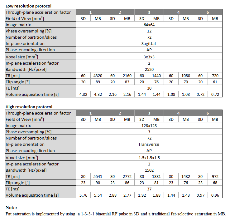
Extensive phantom-based studies were carried out, and findings were confirmed in vivo in a healthy volunteer, on a 3T Tim TRIO (Siemens Healthcare, Erlangen, Germany). 2D-MB-EPI scans were acquired with the gradient echo EPI sequence from the Center for Magnetic Resonance Research (R014 for VB17A, https://www.cmrr.umn.edu/multiband/) while 3D-EPI-CAIPI scans were acquired with an in-house sequence [1]. 10 protocols were tested for each sequence, including low (3mm isotropic) and high (1.5mm isotropic) spatial resolution with a range of acceleration factors (1, 2, 3, 4 and 6) in the through-plane direction. The 2D-MB-EPI sequence uses the CAIPIRINHA sampling scheme, (PE shift = FOV/4) [2]. Therefore, we additionally implemented this sampling scheme into the 3D-EPI sequence [3]. All possible CAIPIRINHA shifts Δ for 3D-EPI-CAIPI were tested and the best (evidenced by maximal temporal signal-to-noise ratio (tSNR) and minimal geometry factor in the phantom) was selected for the final comparison with 2D-MB-EPI. To ensure a maximally fair comparison, the sequence parameters of the two approaches were matched insofar as possible and are summarized in Fig.1. The TR-specific Ernst angle, assuming a T1 value of 1s, was calculated for each sequence. For each protocol, 100 volumes were acquired and respiration and cardiac traces were recorded. All analyses were conducted in SPM12 (www.fil.ion.ucl.ac.uk/spm) using the General Linear Model framework. In brief, each time series was realigned and co-registered to a T1-weighted anatomical image. A grey matter (GM) mask was created by segmenting the anatomical image (P(GM) > 0.6). For time series analysis, the design matrix was composed of a mean term, one linear regressor to model scanner drift and optionally contained physiological regressors for the in vivo data. A high-pass filter with cut-off frequency 1/128 Hz was used. The tSNR of each series was calculated, for voxels within the GM mask, as the estimated parameter of the constant effect divided by the standard deviation of the model residuals.Results
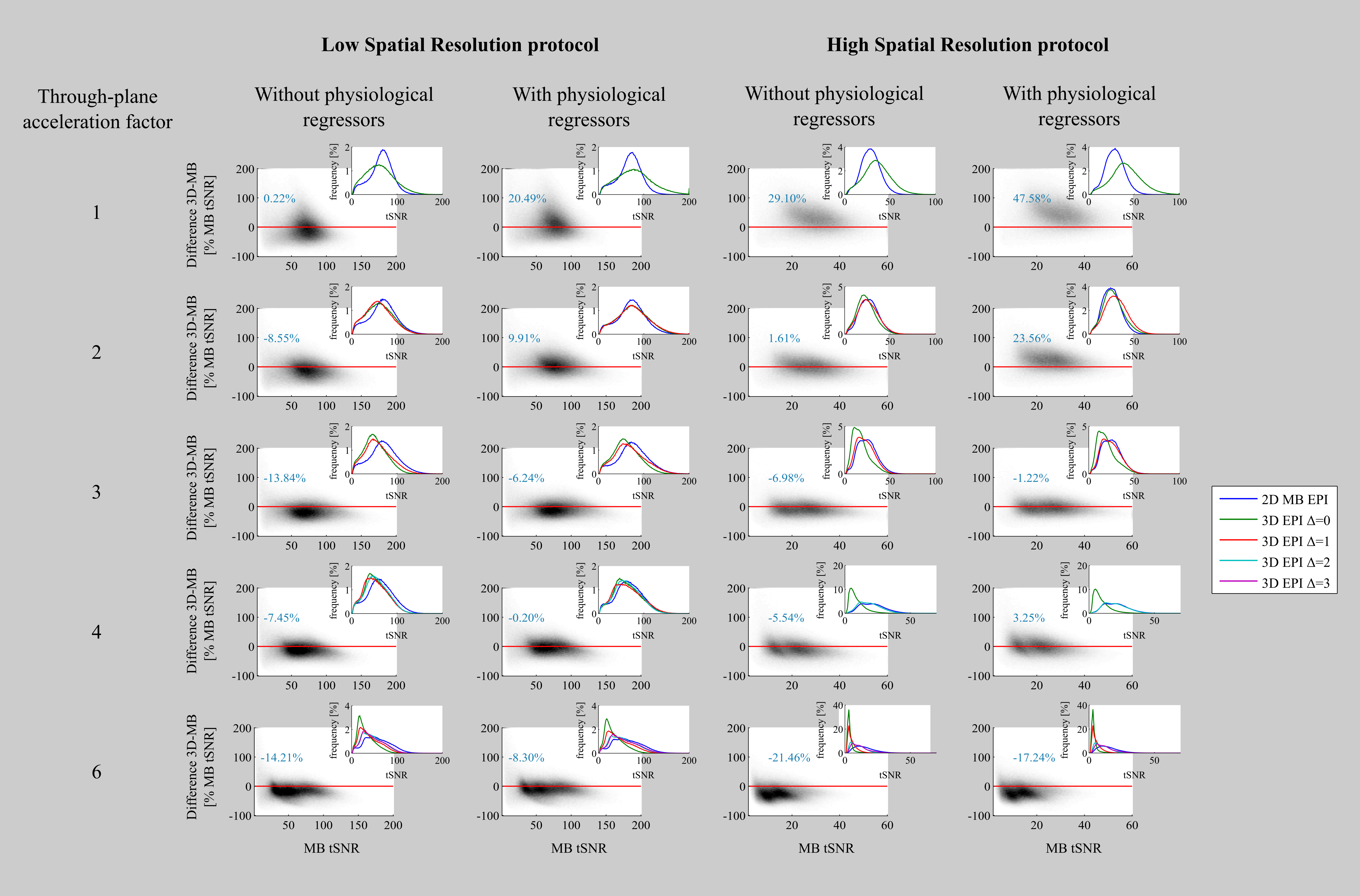
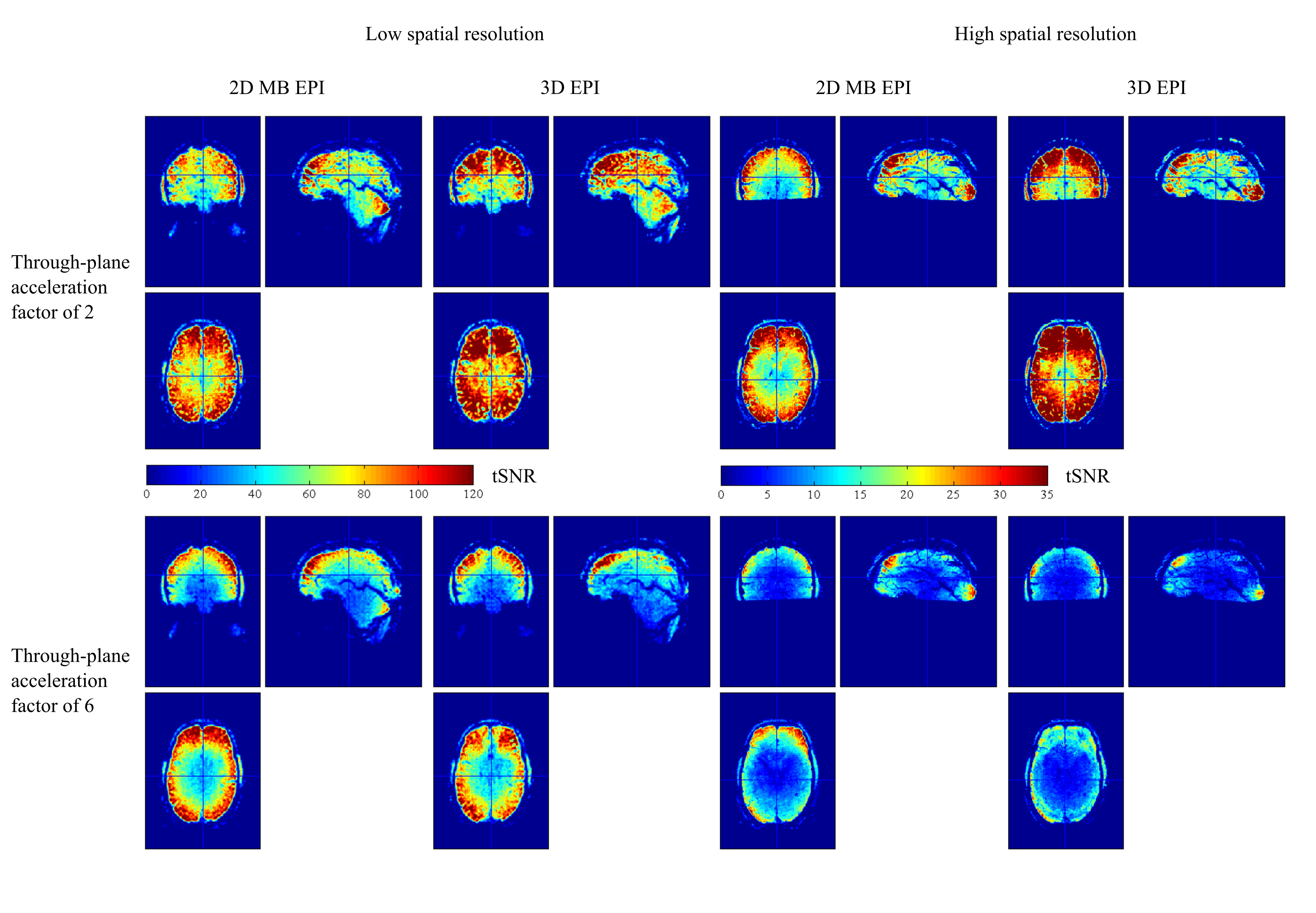
For 3D-EPI-CAIPI the tSNR increased with increasing CAIPIRINHA shift Δ, (histograms inset in Fig.2), especially for high spatiotemporal resolution. Therefore, the maximal was used in the comparison with 2D-MB-EPI (Bland-Altmann plots, Fig.2). At lower spatial resolution (Fig.2, columns 1, 2), the tSNR of 3D-EPI-CAIPI is higher than that of 2D-MB-EPI when physiological regressors are included in the design matrix. At higher temporal resolution, 2D-MB-EPI tends to outperform 3D-EPI-CAIPI. At higher spatial resolution (Fig.2, columns 3, 4), the benefit of 3D-EPI-CAIPI at low acceleration factors is much greater. However, as for lower spatial resolution, the benefit decreases with increasing temporal resolution and for the highest acceleration factor, 2D-MB-EPI offers higher tSNR than 3D-EPI-CAIPI. tSNR maps of series acquired at low and high temporal resolution visually confirm these results (Fig.3).Discussion
Unlike [4], here we matched acquisition parameters (spatial resolution, coverage, bandwidth, TE, in-plane and through-plane acceleration), resulting in approximately equal volume sampling rates for the two approaches. Regardless of spatial resolution, at low acceleration the tSNR of 3D-EPI-CAIPI is higher than that of 2D-MB-EPI, as long as physiological noise is accounted for. As the temporal resolution increases, the tSNR of 3D-EPI-CAIPI decreases more rapidly, such that for high acceleration factors the 2D-MB-EPI approach provides higher tSNR. As the voxel size is decreased, the tSNR of 3D-EPI-CAIPI decreases to a lesser degree than that of 2D-MB-EPI, which is consistent with the results provided by [5] for one acceleration factor.Limitations
Although special effort has been made to match acquisition parameters, the two sequences utilise different reconstruction algorithms. 3D-EPI-CAIPI uses an in-house SENSE-based algorithm implemented in Gadgetron [6], whereas 2D-MB-EPI utilises the split-slice GRAPPA-based algorithm provided with the sequence [7]. The 3D-EPI-CAIPI and 2D-MB-EPI protocols had equivalent sampling rates, however, any differences in the nature of their temporal auto-correlations can be expected to differentially impact their functional sensitivity. Finally, while tSNR is generally accepted as a useful measure of functional sensitivity, further work is needed to confirm that these findings hold in task-based fMRI.Conclusion
For 3D-EPI-CAIPI, it is important to correct for physiological effects and maximally exploit the CAIPIRINHA sampling scheme. Under these conditions, 3D-EPI-CAIPI is the favoured approach for lower through-plane acceleration factors, particularly with higher spatial resolution. As temporal resolution is increased (e.g. < 1s) 2D-MB-EPI is preferred.Acknowledgements
The Wellcome Trust Centre for Neuroimaging is supported by core funding from the Wellcome Trust 091593/Z/10/Z.References
[1]. A. Lutti, D. L. Thomas, C. Hutton, and N. Weiskopf, “High-resolution functional MRI at 3 T: 3D/2D echo-planar imaging with optimized physiological noise correction,” Magn. Reson. Med., vol. 69, no. 6, pp. 1657–1664, Jun. 2013.
[2]. K. Setsompop, B. A. Gagoski, J. R. Polimeni, T. Witzel, V. J. Wedeen, and L. L. Wald, “Blipped-controlled aliasing in parallel imaging for simultaneous multislice echo planar imaging with reduced g-factor penalty,” Magn. Reson. Med., vol. 67, no. 5, pp. 1210–1224, May 2012.
[3]. M. Narsude, D. Gallichan, W. van der Zwaag, R. Gruetter, and J. P. Marques, “Three-dimensional echo planar imaging with controlled aliasing: A sequence for high temporal resolution functional MRI,” Magn. Reson. Med., vol. 75, no. 6, pp. 2350–2361, Jun. 2016.
[4]. R. Stirnberg, Huijbers, B. A. Poser, and T. Stocker, “Ultra-fast gradient echo EPI with controlled aliasing at 3T: simultaneous multi-slice vs. 3D-EPI,” presented at the ISMRM 24th Annual Meeting, Singapore, 2016, p. 0941.
[5]. L. Huber et al., “Blood volume fMRI with 3D-EPI-VASO: any benefits over SMS-VASO? presented at the ISMRM 24th Annual Meeting, Singapore, 2016, p. 0944.
[6]. M. S. Hansen and T. S. Sørensen, “Gadgetron: an open source framework for medical image reconstruction,” Magn. Reson. Med., vol. 69, no. 6, pp. 1768–1776, Jun. 2013.
[7]. S. F. Cauley, J. R. Polimeni, H. Bhat, L. L. Wald, and K. Setsompop, “Interslice leakage artifact reduction technique for simultaneous multislice acquisitions,” Magn. Reson. Med., vol. 72, no. 1, pp. 93–102, Jul. 2014.
Figures