Synopsis

Multi-Spectral Imaging techniques have been shown to significantly reduce metal-induced artifacts. However, they often suffer from residual pile-up and ripple artifacts in the vicinity of metal, where the metal-induced off-resonance gradient “cancels” the frequency-encoding gradient. Fully phase-encoded methods can overcome the drawbacks of frequency encoding, but usually incur prohibitively long scan times. Here we address this limitation by combining two acquisitions with alternating-sign readout and slice-select gradients. We demonstrate with simulations, phantom and in-vivo scans that the proposed method can effectively suppress pile-up and ripple artifacts, and reduce the signal loss areas near the implants.

Purpose

Methods

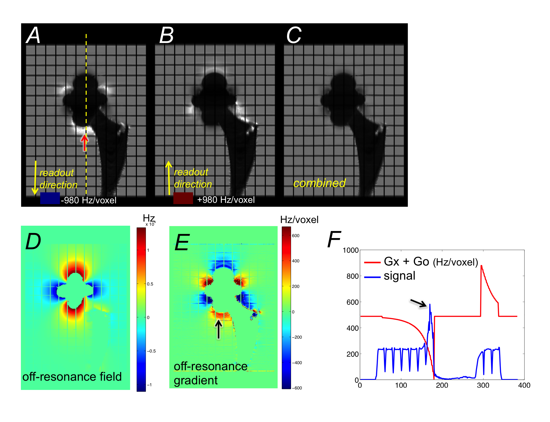
As shown previously³ and in Fig.1 A&B (described in results), pile-ups/ripples appear where the off-resonance gradient $$$G_o$$$ is opposite to the readout gradient $$$G_x$$$. The reduced magnitude of the effective readout gradient $$$(G_o+G_x) $$$ in these areas expands the encoded pixel size, causing irrecoverable loss of resolution in the readout direction. Additive $$$(G_o+G_x)$$$ reduces the encoded pixel size, but its effect can be mostly corrected by deblurring⁸ and Jacobian correction⁵. With the readout gradient $$$G_x$$$ inverted, these artifacts appear in different locations, which can be exploited to suppress pile-up/ripple artifacts.

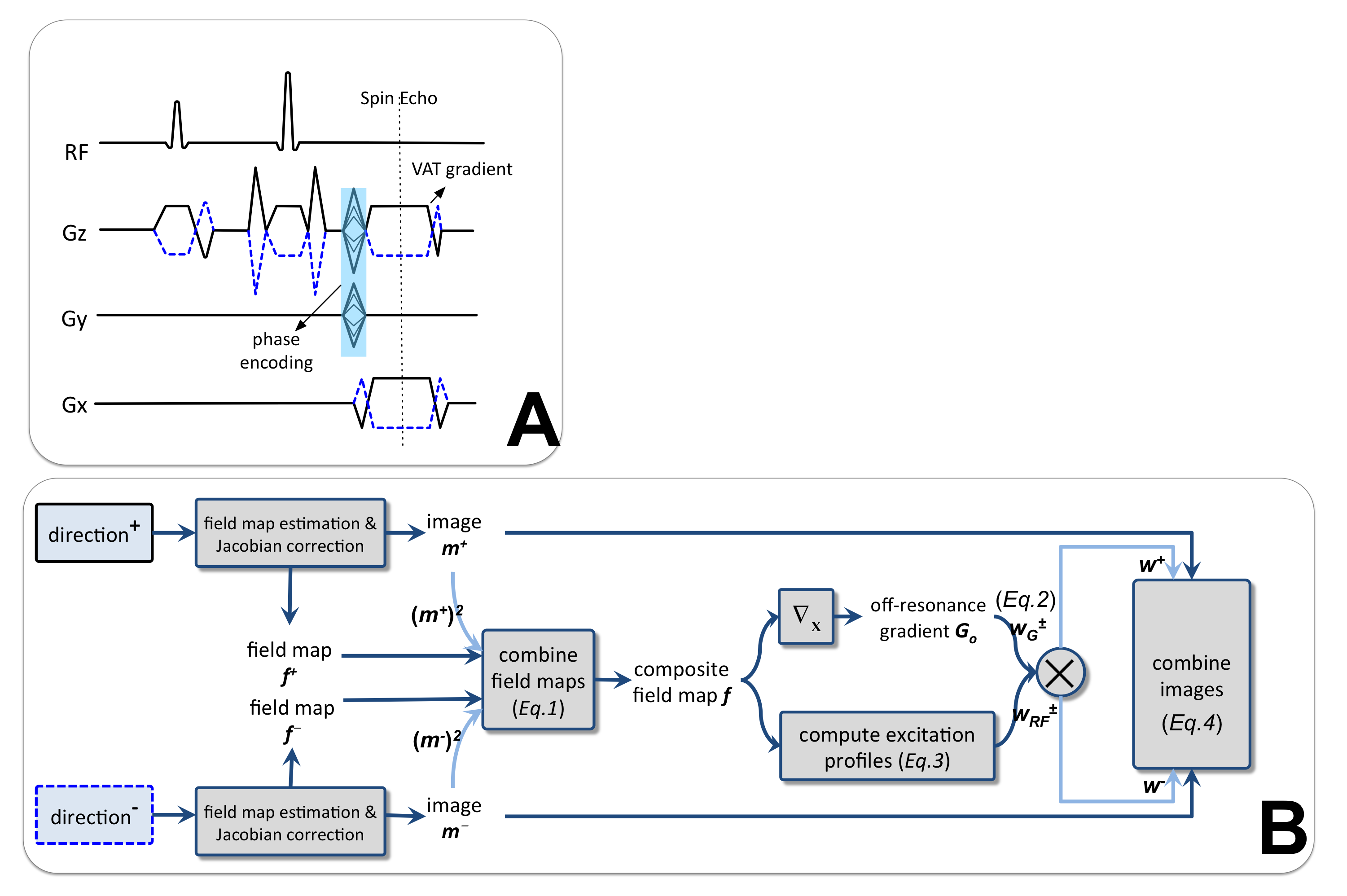
The voxel shearing effect caused by view-angle tilting (VAT), used with selective MSI, can be matched between the two gradient directions by additionally inverting the slice-select and VAT gradients $$$G_z$$$ (Fig.2A), which also changes the regions of non-excited signal loss.

A combination that exploits the different locations of pile-up artifacts and non-excited regions is outlined in Fig.2B:

1. Standard field map estimation, deblurring⁸ and Jacobian correction⁵ are performed separately for images from each gradient direction. The resulting field maps and composite images are denoted as $$$f^+,f^-$$$ and $$$m^+,m^-$$$ , where + and - denote the different gradient directions.

2. A composite field map $$$f$$$ is obtained by combining two field maps:

$$f=[(m^+)^2f^++(m^-)^2f^-]/[(m^+)^2+(m^-)^2]\hspace{10mm}(\mathrm{Eq.1})$$

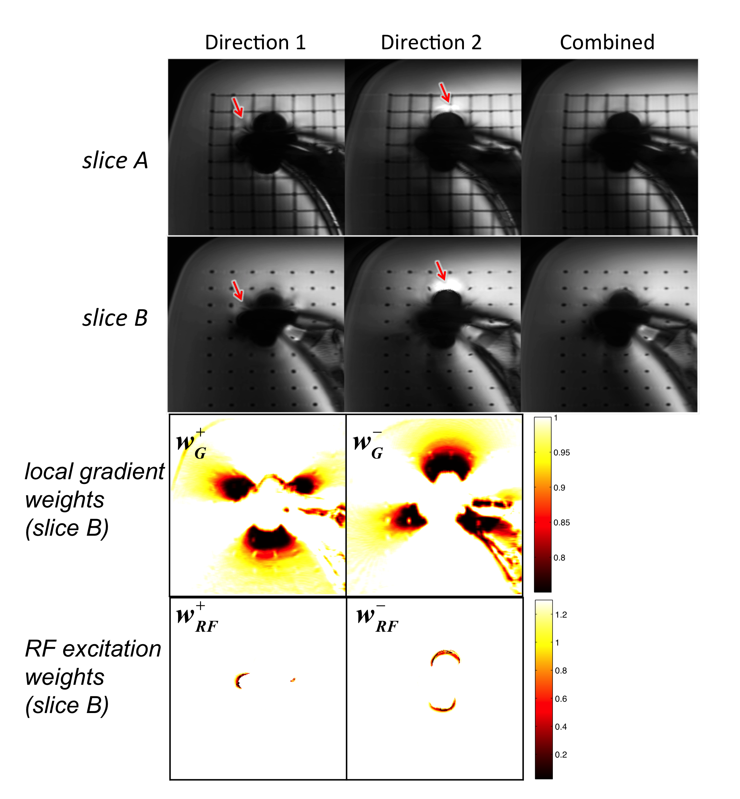
3. The off-resonance gradient $$$G_o$$$ is computed as the finite difference of $$$f$$$ along the readout direction. The local gradient weights of each gradient direction (Fig.3 row3) are computed as

where lower values indicate more severe pile-ups.

4. RF excitation weights (Fig.3 row4) are computed as

$$w_{RF}^±(x,y,z)=\Sigma_b{R_b^2(f(x,y,z)±\gamma\kern-0.6em-G_zz)}\hspace{10mm}(\mathrm{Eq.3})$$

where $$$R_b(\cdot)$$$ represents RF frequency profile of bin b. Lower values indicate non-excited regions.

5. The weighted image combination is

$$f=(w^+m^++w^-m^-)/(w^++w^-)\hspace{10mm}(\mathrm{Eq.4})$$

where the overall weights $$$w^±=\exp\{\alpha w_G^±+\beta w_{RF}^±\}\hspace{2mm}(\mathrm{Eq.5})$$$, scaling factors $$$\alpha=4$$$ and $$$\beta=10$$$ are selected empirically.

The proposed method was validated with simulations with a digital phantom, and MAVRIC-SL scans of a hip implant phantom and volunteers with knee and hip implants. All scans were performed on GE 3T MRI systems with 24 spectral bins spanning ±12kHz, and ±125kHz readout bandwidth. In each scan, the original MAVRIC-SL sequence was run first, and then repeated with readout, slice-select and VAT gradients all inverted. For volunteer scans, translational registration was performed before the combination. The final image reconstructed with the proposed method was compared with the images $$$m^+$$$ and $$$m^-$$$ at step 1.

Results & Discussion

In the simulated acquisition, the proposed combination restored image resolution in areas where pile-up artifacts and blurring were seen in the source acquisitions (Fig.1). The lower signal intensity regions due to additive $$$G_o+G_x$$$, while not reconstructed perfectly, were corrected reasonably well from deblurring and Jacobian correction. Low-signal regions compromised visualization of structures near implants less than pile-up or ripple artifacts.

In the phantom (Fig.3), areas of pile-ups/ripples and non-excited signal loss in images from individual gradient directions were identified by the corresponding combination weights and suppressed in the combined image. The resolution grid in the combined image had the same level of sharpness as each gradient direction’s image, indicating that no additional blurring was introduced by the combination.

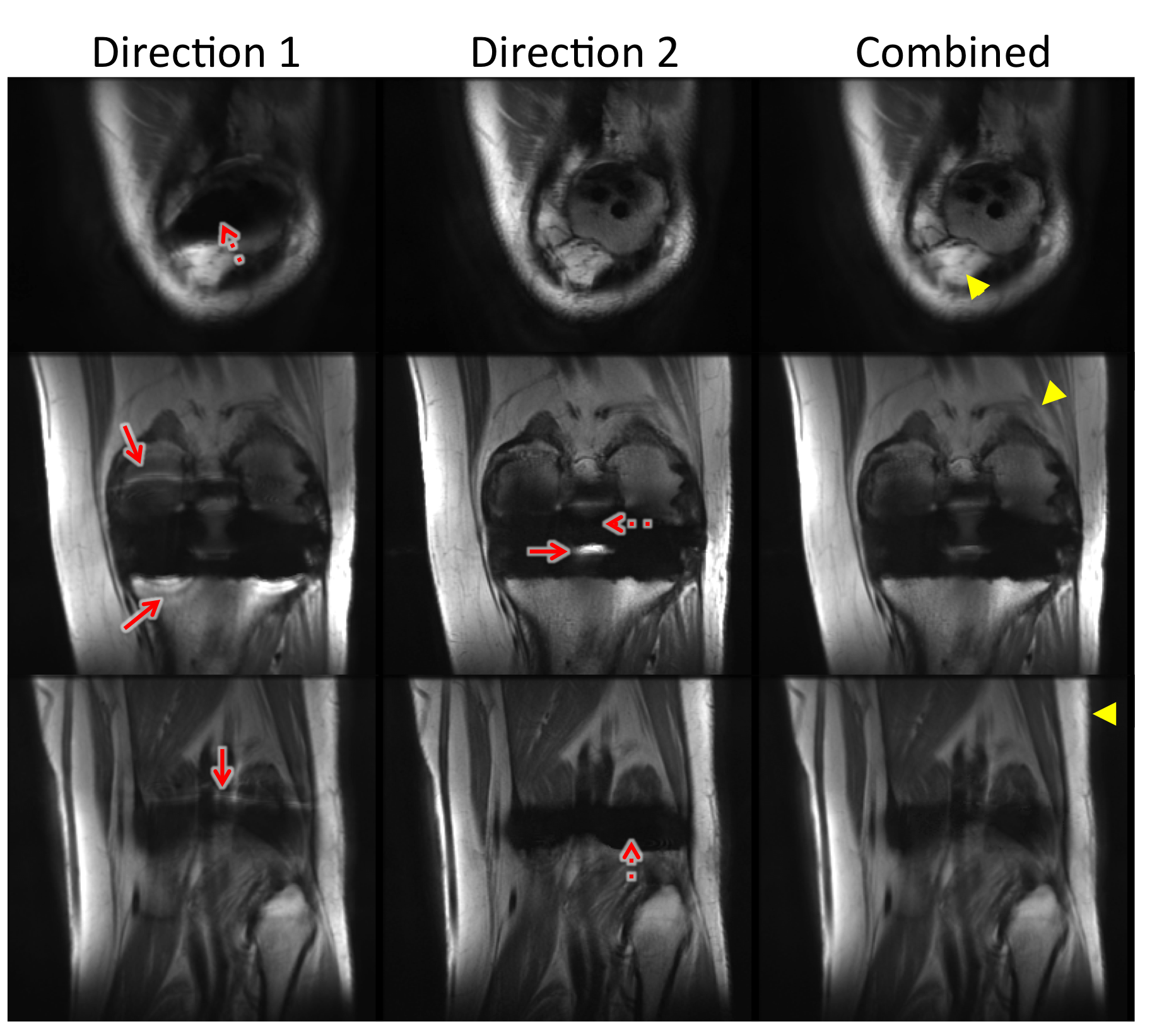
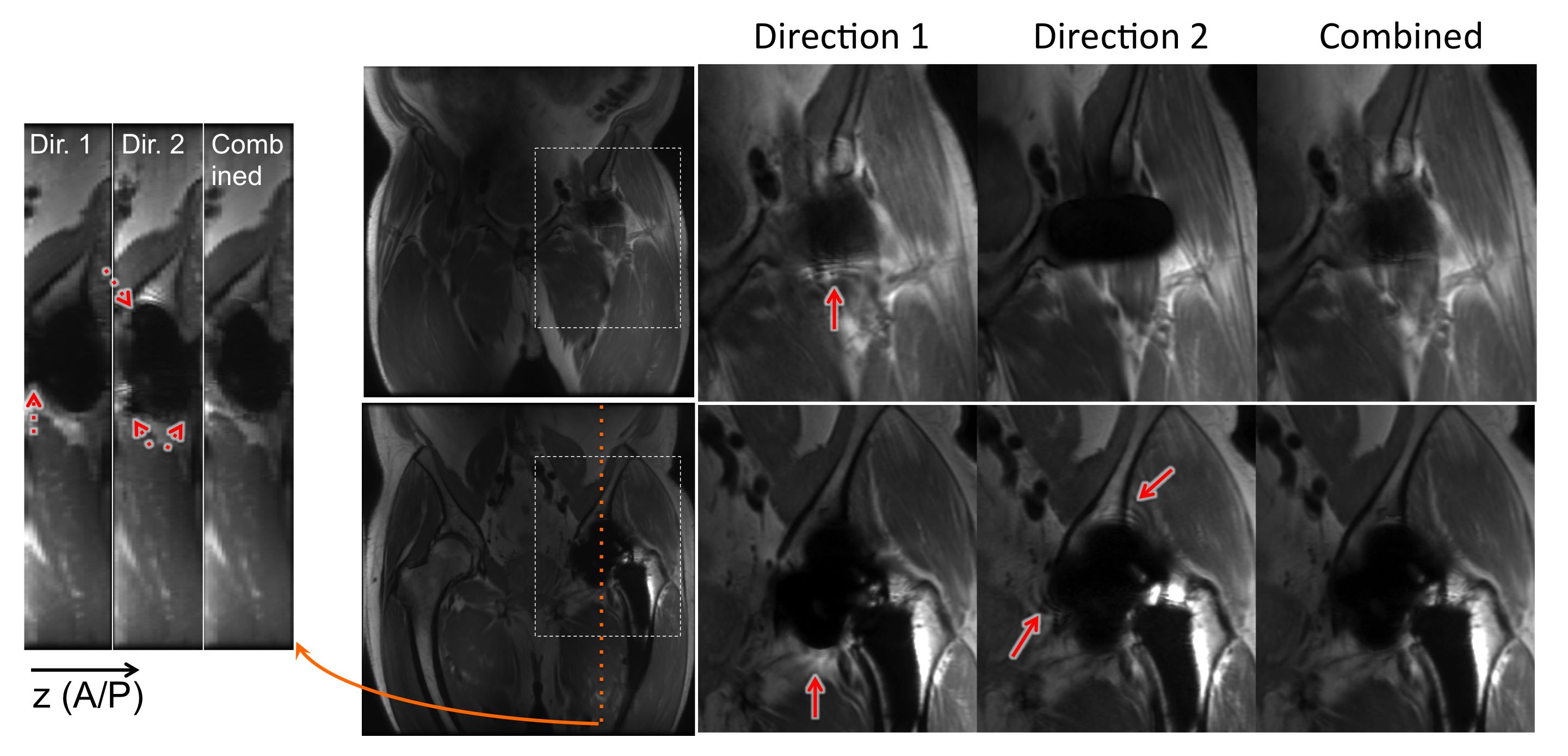
The in-vivo knee and hip results (Figs.4&5) both demonstrated that the proposed combination effectively suppressed the pile-ups/ripples that obscured the underlying structures near the implants. The artifact suppression in combined images was always at least as good as that of either direction, and usually better than both. In these two cases, images of one gradient direction had fewer pile-ups/ripples than the other. But the “better” gradient direction (with smaller artifacts) depends on the specific device/orientation and is unknown before the acquisition, so it cannot be reliably chosen in advance.

A penalty of the proposed method is the doubled scan time. Patient motion during this long scan time may cause blurring in the combined image, and slight blurring of fine structures was observed (arrowheads in Fig.4). In future work, accelerating the acquisitions^9-11 will be explored, as well as schemes to interleave acquisitions and exploit redundancies.

Conclusion

Acknowledgements

References