0554
Low Rank Compressed Sensing Reconstruction for More Precise Cardiac MRF Measurements1Biomedical Engineering, Case Western Reserve University, Cleveland, OH, United States, 2Radiology, University Hospitals, Cleveland, OH, United States
Synopsis
A low rank compressed sensing and parallel imaging reconstruction termed Sparse MRF is introduced to improve the precision of mapping myocardial T1 and T2 with MR Fingerprinting. Sparse MRF enforces data consistency while also constraining the temporal signal evolutions using a low dimensional subspace derived from the SVD of the dictionary along time. Different reconstruction parameters are investigated in simulations with a cardiac phantom. Results from phantom and in vivo cardiac scans indicate that Sparse MRF yields approximately the same mean T1 and T2 measurements as other MRF matching techniques but with smaller standard deviations.
Purpose
MR Fingerprinting (MRF)1-3 can provide quantitative maps of myocardial relaxation times. However, reported values3 for cardiac MRF have a larger spread compared to some conventional mapping sequences. In its original implementation, maps were generated by dot product matching or iterative multi-scaling matching (IMS-MRF)4. However, the dictionary is highly compressible, and several low rank reconstructions have emerged recently5,6. This work aims to improve the precision of cardiac MRF using a low rank compressed sensing and parallel imaging reconstruction that we have called Sparse MRF.Methods
Sparse MRF constrains the temporal signal evolutions using the dictionary according to
$$ min \frac{1}{2}\parallel y-FSU_Kx\parallel_2^2+\lambda\parallel W(U_Kx)\parallel_1$$
The left-hand term enforces data consistency where y is the undersampled k-space, F is the non-uniform FFT, S denotes the coil sensitivities, and x is the MRF images. The projection matrix UK is obtained by compressing the dictionary along time using the SVD6 and retaining the first K rows of U. The MRF images are projected onto a subspace spanned by the dictionary after multiplication by UK and are termed "coefficient images", similar to [7]. An additional L1 wavelet penalty is applied to the coefficient images. The optimization was implemented using a nonlinear conjugate gradient with backtracking line-search routine in MATLAB. It was run for a maximum of 200 iterations or until the relative change in the objective function fell below 0.1%. In the final step, parameter maps were obtained by dot product matching.
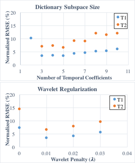
Simulations were performed using the MRXCAT cardiac phantom8 with a simulated 8-channel sensitivity map. Reconstructions were tested with different amounts of dictionary compression (K from 2 to 10 temporal coefficients) and wavelet regularization (λ=0,0.01,0.02,0.03 relative to the maximum intensity in the coefficient images). The normalized RMSE in the T1 and T2 maps was computed for each case. A 5-heartbeat ECG-triggered MRF sequence was simulated with 50 timepoints per heartbeat, 255ms scan window, TR=5.1ms, FA=4-25deg, and a constant 60bpm heart rate.
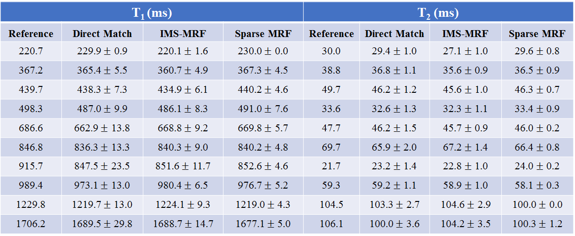
Next an imaging study was performed using a phantom with known T1 and T2 values from inversion recovery and spin echo on a 3T Siemens Skyra with an 18-channel brain coil. Parameter maps were generated by: (1) direct (non-iterative) matching, (2) IMS-MRF with Gaussian lowpass filter widths of 10%, 25%, 75% kmax for the first three iterations and no filtering for the last three iterations, and (3) Sparse MRF with K=5 temporal coefficients and wavelet λ=0.01. Short-axis cardiac scans were also performed in fifteen healthy volunteers at 1.5T (Siemens Aera) in an IRB-approved HIPAA-compliant study using a 15-heartbeat ECG-triggered MRF sequence3, and maps were reconstructed as in the phantom study.
Results
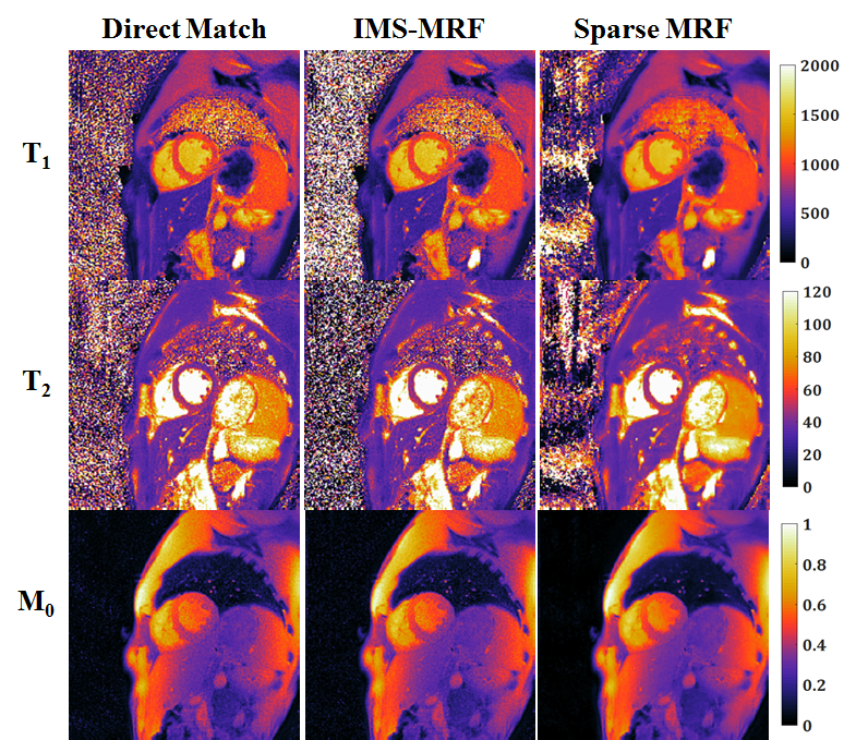
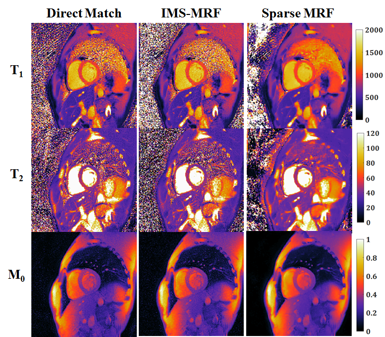
From simulations (Fig 1), the smallest errors in the T1 and T2 maps were obtained with five temporal coefficients (RMSE 3.5% T1, 6.5% T2). Larger RMSEs were recorded with fewer than three and more than six coefficients. More accurate parameter maps were obtained with a small wavelet penalty (λ=0.01) applied to the coefficient images. Table 1 shows the mean and standard deviations for T1 and T2 within each phantom tube. Sparse MRF yielded approximately the same mean values as dot product matching and IMS-MRF but with smaller standard deviations. The average reconstruction times including gridding and pattern matching were 9s direct matching, 138s IMS-MRF, and 549s Sparse MRF. Representative in vivo maps are shown in Figures 2 and 3. Myocardial T1 and T2 measurements are more homogeneous in the Sparse MRF maps. Myocardial wall measurements pooled over all volunteers yielded dot product matching T1 952+/-106ms and T2 44.2+/-6.3ms, IMS-MRF T1 961.9+/-110.0ms T2 44.6+/-6.4ms, and Sparse MRF T1 995+/-69ms and T2 46.8+/-4.3ms. Additionally, in vivo maps were reconstructed using only the first 5 heartbeats from the 15-heartbeat scan, which yielded dot product matching T1 987+/-101ms and T2 45.7+/-9.4ms, IMS-MRF T1 1001.9+/-107.7ms and T2 46.1+/-10.1ms, and Sparse MRF T1 1018+/-64ms and T2 47.1+/-5.9ms.Discussion
Sparse MRF combines compressed sensing and parallel imaging to denoise aliased MRF images before pattern matching, which enables more precise mapping of myocardial relaxation times. Sparse MRF does require long computation times of approximately 10min in MATLAB without GPU acceleration. Comparing Sparse MRF to direct matching in the volunteer study, the standard deviation over the myocardial wall decreased by 35% for T1 (106ms to 69ms) and 32% for T2 (6.3ms to 4.3ms) without appreciably different mean T1 or T2 measurements. Sparse MRF exploits the low rank properties of the dictionary, which can be described with a few temporal basis coefficients.Conclusion
Sparse MRF can be used to obtain more precise measurements of myocardial T1 and T2 by combining compressed sensing, parallel imaging, and MR Fingerprinting.Acknowledgements
Siemens Healthcare, NIH/NHLBI R01HL094557.References
1. Ma D, Gulani V, Seiberlich N, et al. Magnetic resonance fingerprinting. Nature 2013;495:187–92.
2. Jiang Y, Ma D, et al. MR fingerprinting using fast imaging with steady state precession (FISP) with spiral readout. Magn Reson Med 2014;74:1621–1631.
3. Hamilton JI, Jiang Y, et al. MR fingerprinting for rapid quantification of myocardial T1, T2, and proton spin density. Magn Reson Med 2016. Early View.
4. Pierre EY, Ma D, et al. Multiscale reconstruction for MR fingerprinting. Magn. Reson. Med. 2016;75:2481–2492.
5. Doneva M, Amthor T, et al. Low Rank Matrix Completion-based Reconstruction for Undersampled Magnetic Resonance Fingerprinting Data. Proc ISMRM 2016, Singapore. Oral 432.
6. McGivney DF, Pierre E, et al. SVD compression for magnetic resonance fingerprinting in the time domain. IEEE Trans. Med. Imaging 2014;33:2311–2322.
7. Tamir JI, Uecker M, et al. T2 shuffling: Sharp, multicontrast, volumetric fast spin-echo imaging. Magn Reson Med 2016. Early View. doi:10.1002/mrm.26102.
8. Wissmann L, Santelli C, et al. MRXCAT: Realistic numerical phantoms for cardiovascular magnetic resonance. J. Cardiovasc. Magn. Reson. 2014;16:63.
Figures