0461
Fibre orientation dispersion in the corpus callosum relates to interhemispheric functional connectivity1FMRIB centre, University of Oxford, Oxford, United Kingdom, 2Department of Anatomy, Donders Institute for Brain, Cognition and Behaviour, Radboud University Medical Centre, Nijmegen, Netherlands
Synopsis
Fibre orientation dispersion was previously demonstrated to be higher at the center compared to lateral aspects of the corpus callosum (CC) using microscopy data and diffusion MRI data. We hypothesize that this pattern of dispersion in the CC relates to the degree of heterotopic connections in the brain. In a large cohort of 4903 subjects from the Biobank UK, resting-state functional MRI and diffusion MRI data were compared against each other to find associations between fibre dispersion and functional interhemispheric connectivity
Purpose
Linking the anatomy of brain connections to function is fundamental to our understanding of how brain architecture underpins human cognition. A prominent set of brain connections, collectively called the ‘corpus callosum’ (CC), plays a key role in cross-hemispheric information transfer. Although the CC is generally thought of as a well-organized bundle of axons running parallel to each other and connecting homologous (homotopic) areas, recent studies have demonstrated complex fibre architecture within the CC1-3. In particular, fibre orientation ‘dispersion’ at the midline appears to be greater, compared to the lateral aspects of the CC4. This deviation from a well-organized CC might reflect interhemispheric connections of non-homologous (heterotopic) areas. Here we hypothesize that dispersion in the CC is indeed a signature of the degree of heterotopic connectivity. We test this hypothesis in a large cohort of subjects by looking for associations between diffusion MRI (dMRI) estimates of fibre dispersion and resting-state functional MRI (rfMRI) estimates of interhemispheric connectivity.Methods
We analyzed dMRI and rfMRI data from 4903 subjects in the UK Biobank project (acquisition parameters and pre-processing steps can be found elsewhere)5.
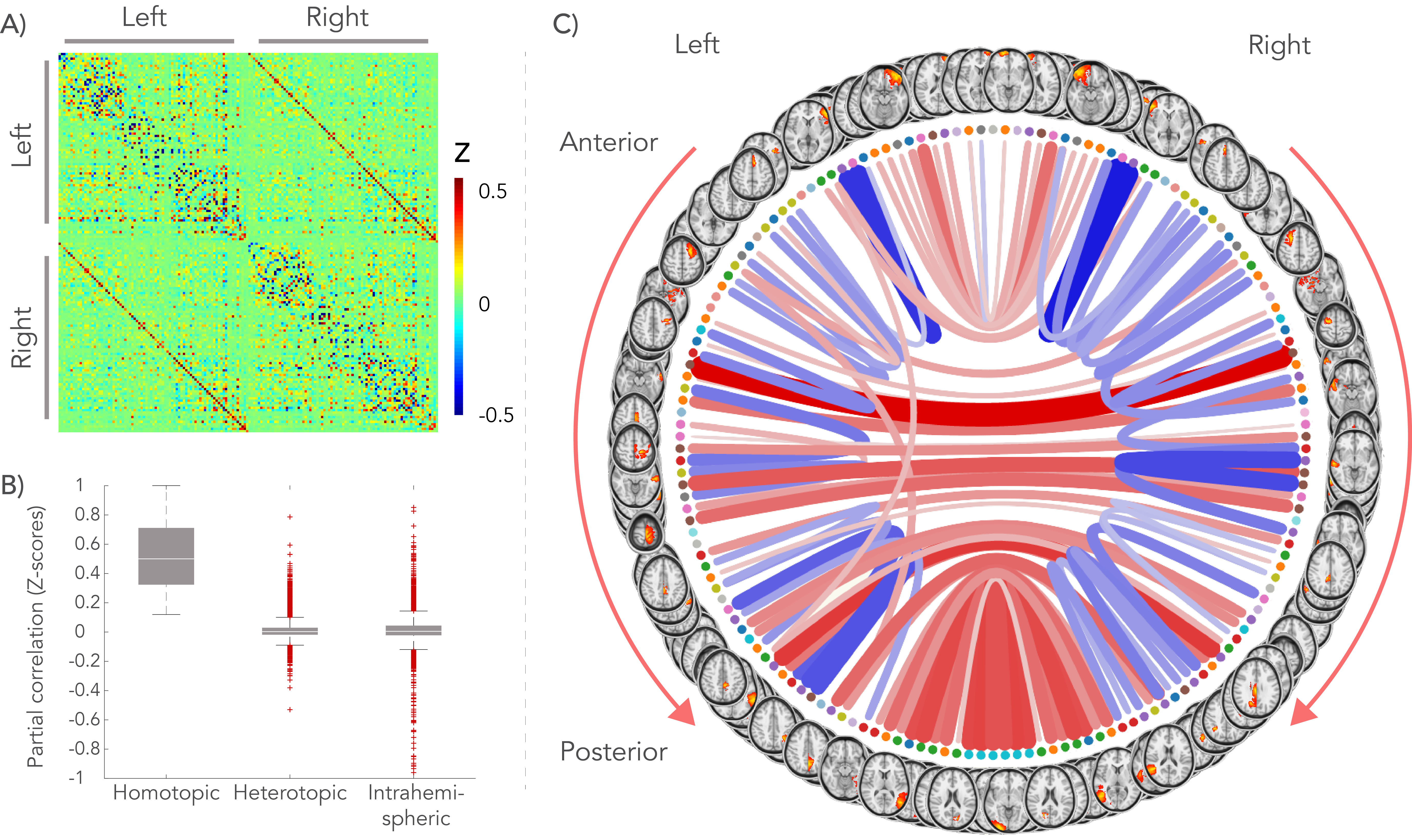
A group-average decomposition of functional connectivity using ICA yielded 55 components corresponding to resting-state networks. These were then split for each hemisphere and possibly further split if a component contained non-contiguous brain areas. To estimate subject-specific connectivity between the resulting brain regions (network ‘nodes’), average time-series were generated for every node and correlated with each other using partial correlation. These connectivity values then form a node-by-node matrix of network connectivity. To quantify the balance of homo- to heterotopic interhemispheric connections for a given node, a functional asymmetry index (AI) was defined as the homotopic connection strength minus the mean of the 10% strongest heterotopic connections.
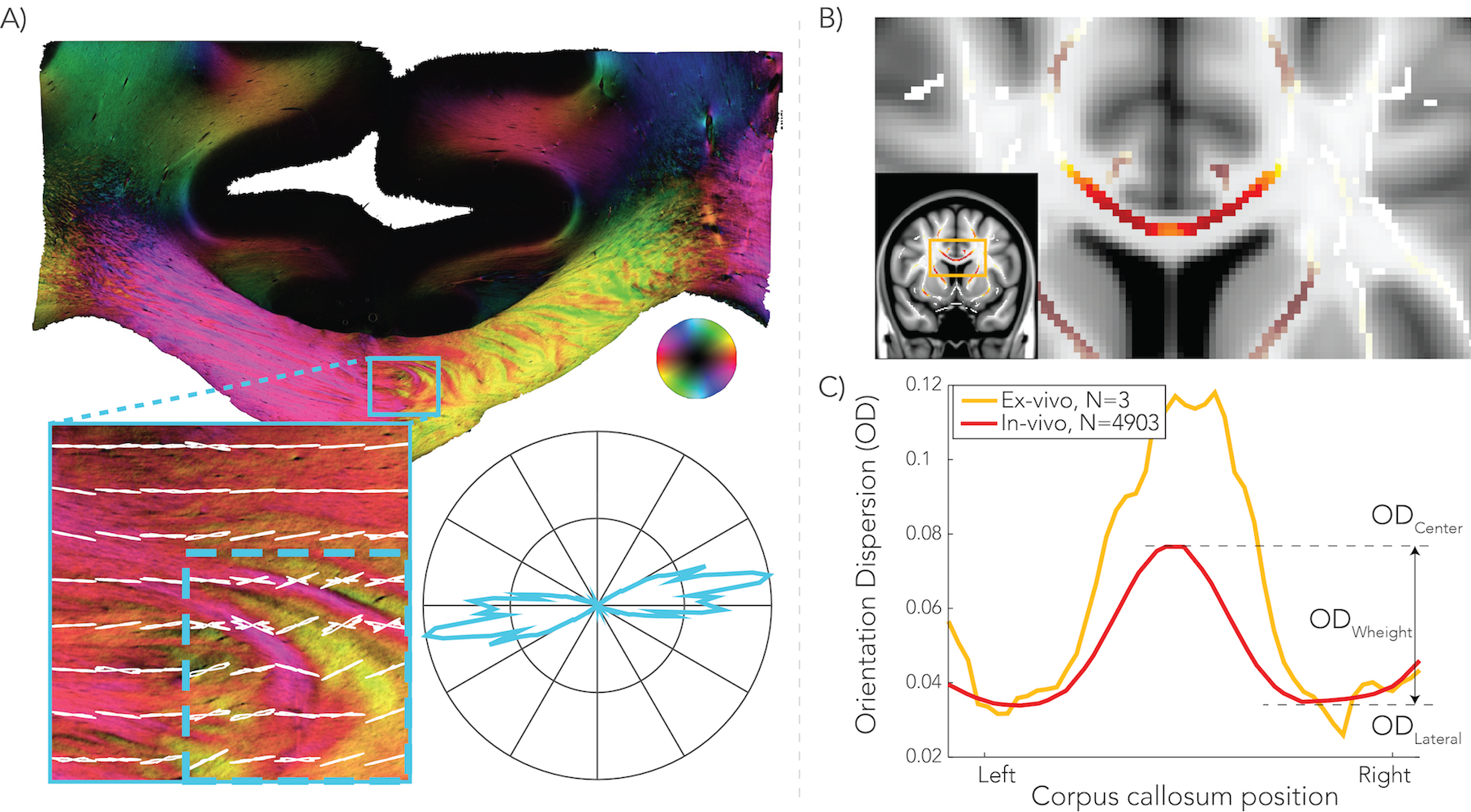
To calculate voxel-wise orientation dispersion (OD), the NODDI model6 was fit to dMRI data using AMICO7. OD values were extracted from the CC after transforming all subjects to the same space and mapping ODs onto a skeleton using TBSS8. To estimate which anterior-to-posterior region of CC connects a pair of homotopic areas, structural connectivity probability maps for each node were obtained in the CC using a tractography template. Dispersion was calculated as the mean OD at the center minus the mean OD at the lateral aspects of the CC, referred to as OD hereafter (Figure 1.C).
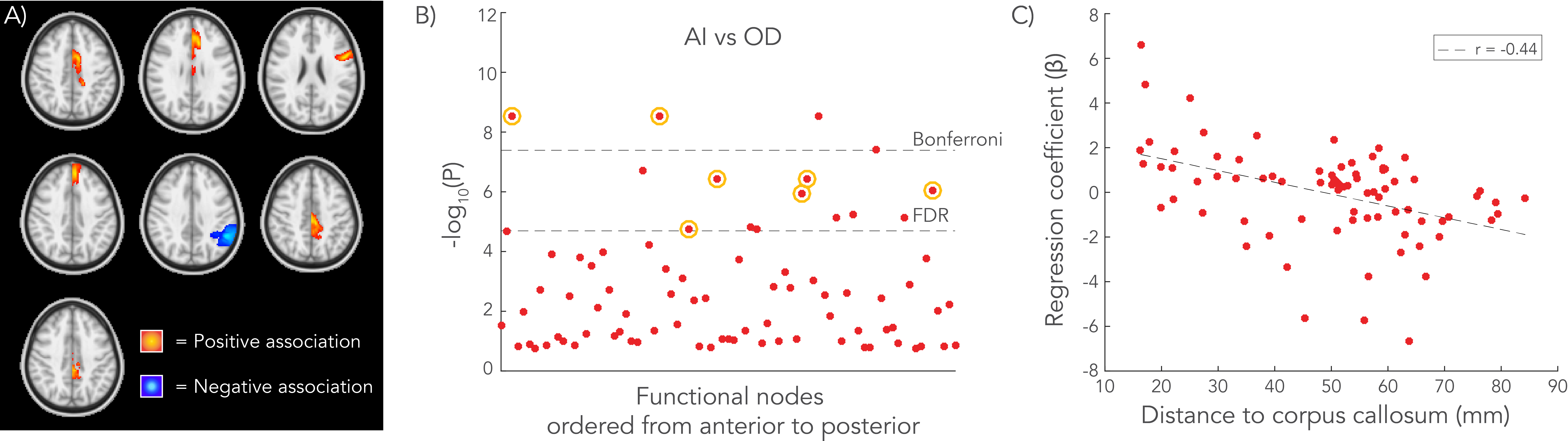
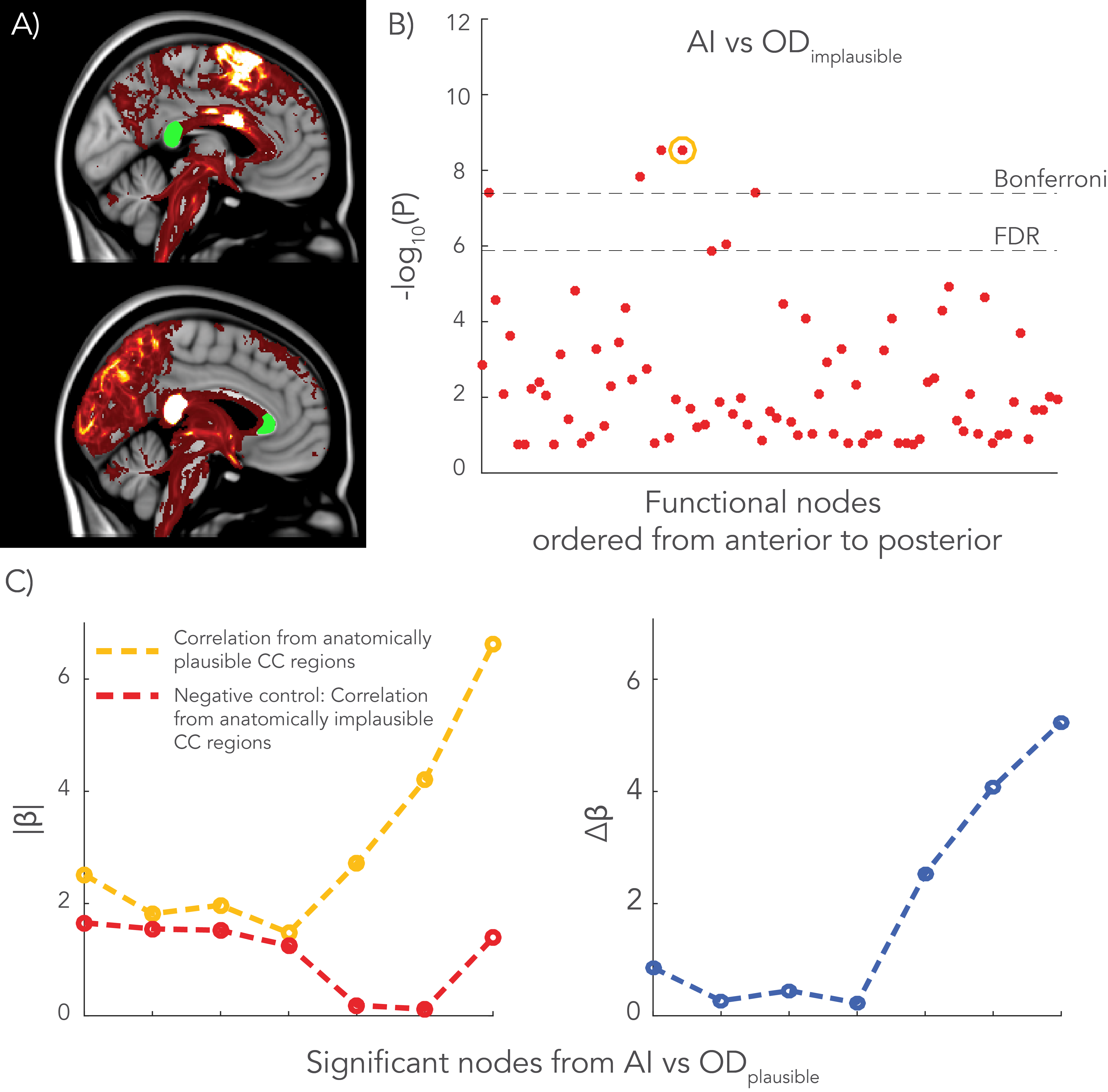
Associations between OD and AI were calculated, with statistical significance assessed using permutation testing (5000 permutations). Reproducibility was demonstrated by dividing the subjects in two equally sized groups with similar gender and age distribution. For each AI vs OD comparison, the OD values were taken from a region of the CC that connects to the cortical node of interest. A negative control analysis was done by correlating AIs with OD derived from the CC region that is least likely to interconnect the node of interest.
Results
As reported previously4, high dispersion was found in the center of the CC in both dMRI data and polarized light imaging, creating a W-shaped pattern (Figure 1). The splenium, however, exhibited an inverted W-profile. Figure 2 illustrates the group-average functional connectome. For each hemisphere, 81 nodes were defined and homotopic connections exhibited the highest correlations.
Significant associations between AI and OD were primarily found near the midline, with correlation coefficients ranging between r=0.05-0.11 (Figure 3). Of 16 significant associations in the “discovery” in the first group of subjects that survive FDR multiple comparison correction, seven were reproduced in the second group. Highest regression coefficients (β) were found closer to the CC, and lower regression coefficients distal to the CC (Figure 3.D).
Finally, the negative control analysis yielded a single significant and reproducible association between AI and OD in an implausible CC region (Figure 4), although with a lower regression coefficient (β=1.55) than the anatomically plausible CC region (β=1.82).
Discussion
The W-shaped OD profile was consistently found in the CC of living subjects. Significant associations were found between AI vs OD in regions close the CC, such as the cingulate cortex. In addition, the AI of a particular area appeared to be less associated with OD if the area was more laterally located. We hypothesize that dispersion in the CC is more crucial for midline nodes to project to nearby heterotopic regions, while nodes that are more distant from the CC can form a path to heterotopic areas via other tracts. The negative control analysis yielded one significant node that may be explained by correlation of ODs among different areas of the CC. It may also relate to an indirect association of an alternate biological source.Acknowledgements
This work was funded by the Wellcome Trust FoundationReferences
1. Mikula S. et al. Staining and embedding the whole mouse brain for electron microscopy. Nature Methods (2012).
2. Ronen I. et al. Microstructural organization of axons in the human corpus callosum quantified by diffusion-weighted magnetic resonance spectroscopy of N-acetylaspartate and post-mortem histology. Brain Structure and Function (2014).
3. Budde M.D. et al. Quantification of anisotropy and fiber orientation in human brain histological sections. Frontiers in integrative neuroscience (2013).
4. Mollink J. et al. Exploring fibre orientation dispersion in the corpus callosum: Comparison of Diffusion MRI, Polarized Light Imaging and Histology. Proceedings ISMRM (2016).
5. Miller K.L. et al. Multimodal population brain imaging in the UK Biobank prospective epidemiological study. Nature Neuroscience (2016).
6. Zhang H. et al. NODDI: Practical in vivo neurite orientation dispersion and density imaging of the human brain. Neuroimage (2012).
7. Daducci A. et al. Accelerated Microstructure Imaging via Convex Optimization (AMICO) from diffusion MRI data. Neuroimage (2015).
8. Smith S.M et al. Tract-based spatial statistics: Voxelwise analysis of multi-subject diffusion data. Neuroimage (2006).
Figures