0435
Water-Only Look-Locker Inversion recovery (WOLLI) T1 mapping1OCMR, RDM Cardiovascular Medicine, University of Oxford, Oxford, United Kingdom, 2Translational Gastroenterology Unit, Nuffield Department of Medicine, University of Oxford, Oxford, United Kingdom, 3Oxford Centre for Diabetes, Endocrinology and Metabolism (OCDEM), Radcliffe Department of Medicine, University of Oxford, United Kingdom
Synopsis
We propose a new “Water-Only Look-Locker Inversion recovery” (WOLLI) sequence, based on MOLLI, that enables water-selective T1-mapping in an 8hb breath-hold at 3T. WOLLI uses a hypergeometric (HG) inversion pulse to selectively invert water with negligible effect on fat. To separate the steady-state fat and water signals, WOLLI adds one or more fat-inversions starting from the plateau of the water T1* recovery. WOLLI uses an extended Deichmann-Haase formula to correct for readout-induced saturation. We validated this approach by simulations, scans in a phantom containing 19 fat/water mixtures, and liver scans in 12 subjects (volunteers and liver disease patients).
Purpose
In the liver, T1-mapping can detect the onset of fibrosis or cirrhosis, e.g. using Modified Look-Locker Inversion Recovery (MOLLI) or Shortened MOLLI (ShMOLLI).1,2 But diseased livers often contain intracellular fat – up to 40% in severe cases.3–7 This fat can make MOLLI T1-values deviate substantially from the T1 of water.8,9 We present a new Water-Only Look-Locker Inversion recovery (WOLLI) sequence that maps water T1 even in the presence of fat.Theory
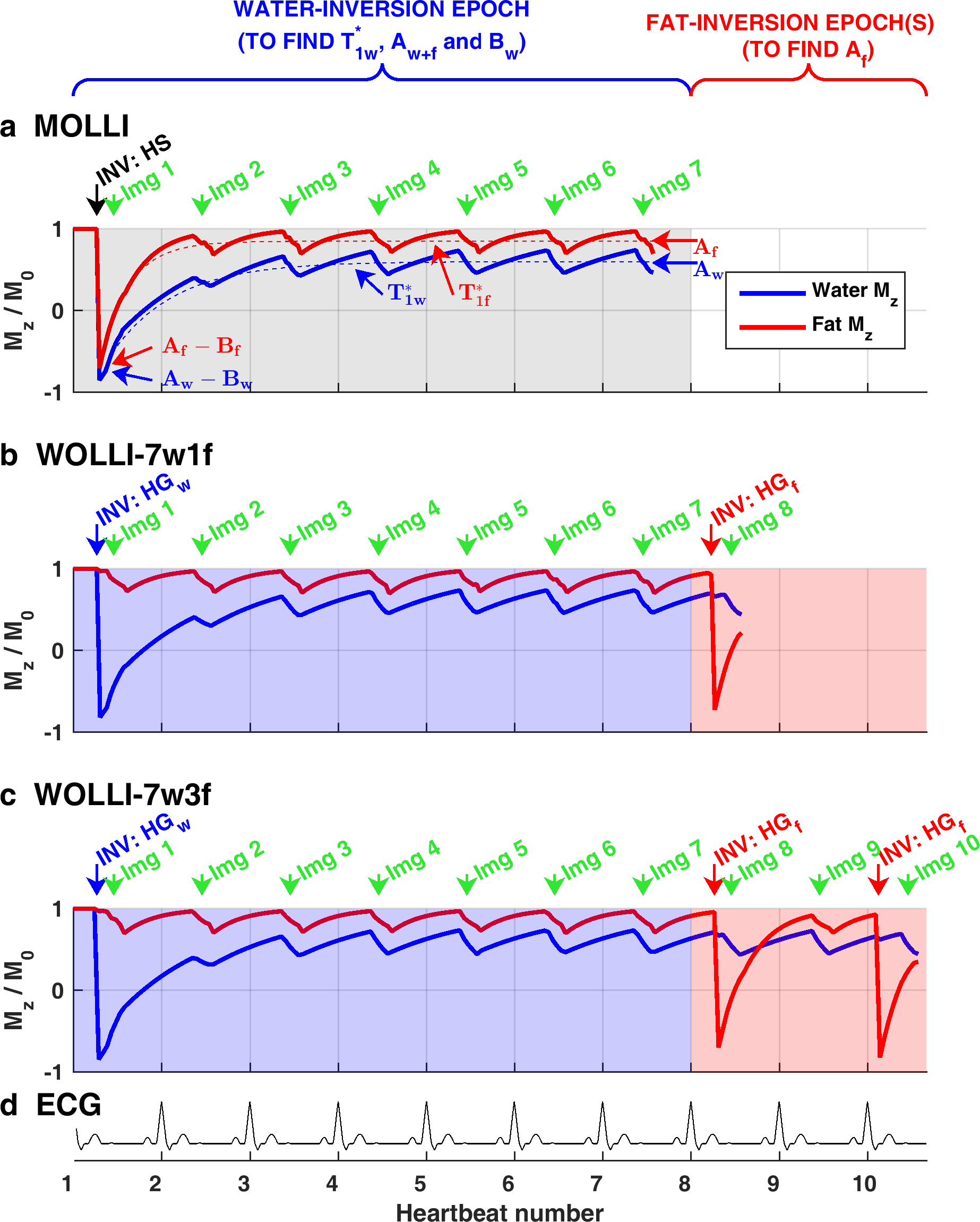
MOLLI (Fig. 1a) uses “inversion epochs” containing a hyperbolic secant (HS) inversion pulse, followed by ECG-gated bSSFP readouts that sample the recovering magnetization in one breath-hold.10,11
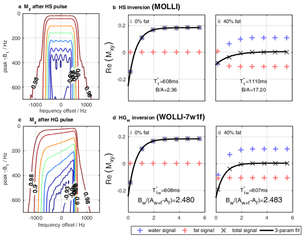
The MOLLI HS pulse (Fig. 2a) inverts magnetization over $$$\gamma\Delta B_0\approx\pm500Hz$$$, which means that fat (offset by 420Hz at 3T) is inverted too.12
We optimized a hypergeometric13 (HG) pulse (Fig. 2c) that has a similar duration, SAR and adiabatic onset to MOLLI's HS pulse. But the HG pulse is asymmetric, sharpening the transition-width between fat and water, enabling fat or water to be inverted selectively.
The complex-valued signal in a voxel containing water and fat (at fat fraction Ff) is
$$S_{\mathrm{SSFP}}=(1-F_f)\times M_{SS,w}(T_{1,w},T_{2,w},\gamma\Delta B_0-\nu_\mathrm{w})+F_f\times M_{SS,f}(T_{1,f},T_{2,f},\gamma\Delta B_0-\nu_\mathrm{f})\quad[1]$$
where subscripts denote water and fat, and $$$M_{SS}$$$ is the bSSFP signal.
MOLLI analysis11 fits A, B, and $$$T_1^*$$$ pixelwise to:
$$S_{\mathrm{TI}}=A-B\exp\left(-\frac{TI}{T_1^*}\right)\quad[2]$$
where $$$TI$$$ is the inversion time, and $$$T_1^*$$$ is an effective relaxation time. The Deichmann-Haase formula14 corrects $$$T_1^*$$$ for readout-induced saturation:
$$T_1^{\mathrm{DH}}=T_1^*(B/A-1).\quad[3]$$
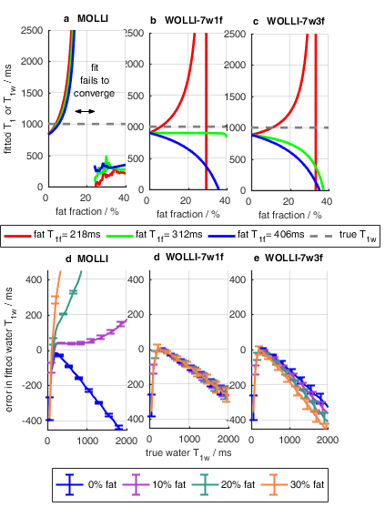
Figure 2b shows the failure of MOLLI and Eqs [2-3] at high fat fractions. Both $$$T_1^*$$$ and $$$B/A$$$ are wrong.
Extending Eq. 2 to allow for selective inversion we write
$$S_{TI_{\mathrm{k}}}=A_\mathrm{k}-B_\mathrm{k}\exp\left(-\frac{TI_\mathrm{k}}{T_{1,\mathrm{k}}^*}\right);\quad\mathrm{where}\ A_k=\mathrm{\alpha}_\mathrm{k}M_{z,k}^\mathrm{SS},\ \mathrm{and}\ B_k=A_k-\mathrm{\alpha}_\mathrm{k}M_{z,k}^+.\quad[4]$$
$$$TI_{\mathrm{k}}$$$ is the time since the most recent interruption of readouts for the kth pool; $$$T_{1k}^*$$$ is apparent relaxation time; $$$A_k$$$ is the $$$T_1^*$$$-recovery plateau signal; and $$$A_k-B_k$$$ is the signal immediately after inversion. Note that this signal depends on the inversion efficiency ($$$IE_k=M_{z,k}^+/M_{z,k}^-$$$) of the inversion pulse, and also on the longitudinal magnetization just before inversion $$$M_{z,k}^-$$$.
Providing the magnetization is at equilibrium before inversion (implicitly assumed in MOLLI), the Deichmann-Haase formula (Eq. 3)14,15 can be extended:
$$T_{1,k}^\mathrm{DH}\approx T_{1,\mathrm{k}}^*/(A_k/\alpha M_{0,k})=T_{1,\mathrm{k}}\left(1-\frac{B_k^{\mathrm{plateau}}}{A_k}\right)/IE_k\quad[5]$$
The inversion efficiency $$$IE_k$$$ is +1 for FA=0°, -1 for FA=180°.
Figure 2d shows that simply swapping HS (global) to HG (water-selective) inversion gives the correct $$$T_{1w}^*$$$, but is insufficient to obtain $$$T_{1w}$$$ because Eq. 5 requires $$$A_w$$$, but the observed steady-state signal $$$A_{w+f}\equiv{}A_w+A_f$$$ comes from both water and fat.
To separate the water $$$A_w$$$ and fat $$$A_f$$$ contributions to the plateau signal, we apply one or more fat-selective-inversion pulse(s) in the middle of a series of readouts at the water $$$T_1^*$$$ plateau. The water signal stays unchanged. But the signal in the fat pool inverts to minus the plateau value, and so $$$A_f=B^\mathrm{SS}_f/2$$$, i.e. half the change in signal after fat-selective inversion. Hence $$$A_w = A_{w+f}-A_f$$$, and is given by Eq. 5.
WOLLI pulse sequence and fitting
WOLLI (Figure 1b-c) applies this concept for water-selective T1 mapping. WOLLI uses water-selective HG inversion and a train of ECG-gated bSSFP readouts, followed immediately by block(s) of fat-selective inversion and more SSFP readout(s). Data are fitted pixel-wise first to the water-inversion data in images #1-#7 to obtain $$$A_{w+f},B_w,\mathrm{\,\,and\,\,}T_{1w}^*$$$. Then the fat-inversion images (#8 onwards) are fitted to separate the contributions $$$A_w$$$ and $$$A_f$$$. Finally, Eq. 5 is used to obtain the water $$$T_{1w}$$$.Methods
Matlab was used for simulations and data-processing.
Two WOLLI protocols were used in this study: WOLLI-7w1f, with one final image at the fat-null after fat-inversion; and WOLLI-7w3f, with three fat-inverted-images at different fat TIs, and we fit $$$T_{1f}^*$$$ in post-processing. We tested the sequence on a 3T Trio (Siemens), on a 19-vial fat-water phantom, and in vivo in the livers of 12 subjects (volunteers and liver disease patients).
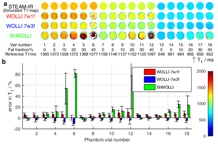
We matched the T1 imaging parameters to a recent a clinical study1, i.e. ShMOLLI 5(1)1(1)1, with 35° FA, 2.51/1.05ms TR/TE, and 1.9x1.9x8.0mm3 voxel size. Reference T1 values were obtained by STEAM-IR single-voxel spectroscopy with TE=10ms, TM=7ms, and TR=2s.
Results
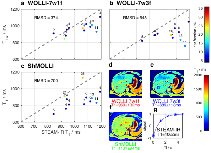
Figure 3 shows simulations comparing T1 accuracy vs fat fraction, $$$T_{1f}$$$, and $$$T_{1w}$$$. For fat fractions from 0 to 40%, T1s varied by: <0.5% (WOLLI-7w1f), <12% (WOLLI-7w3f), and >2000% (MOLLI). In phantoms (Fig. 4), the methods' accuracies (worst-case $$$T_{1w}$$$ difference vs spectroscopy) were: WOLLI-7w1f max. diff. 10.2%, WOLLI-7w3f max. diff. 10.5%, and ShMOLLI max. diff. 81.5%. In vivo (Fig. 5), the root-mean-squared-deviations vs spectroscopy $$$T_{1w}$$$ were: 374 (WOLLI-7w1f), 645 (WOLLI-7w3f), and 700 (ShMOLLI).Conclusion
For tissue with suspected fat infiltration, WOLLI provides an attractive complementary approach to MOLLI. WOLLI is less sensitive to fat, but requires a slightly longer breath-hold and gives slightly lower SNR T1 maps.Acknowledgements
Funded by the Wellcome Trust [098436/Z/12/Z]. We thank William Clarke for Bloch simulation tools and Aaron Hess for helpful discussion. WOLLI is the subject of a provisional US Patent application: US 62/391,202.References
1. Banerjee, R. et al. Multiparametric magnetic resonance for the non-invasive diagnosis of liver disease. J. Hepatol. 60, 69–77 (2014).
2. Neuberger, J. Guidelines on the use of Liver Biopsy in Clinical Practice. BSG Guidel. Gastroenterol. 1–15 (2004). doi:10.1136/gut.45.2008.iv1
3. Takahashi, Y. & Fukusato, T. Histopathology of nonalcoholic fatty liver disease/nonalcoholic steatohepatitis. World J. Gastroenterol. 20, 15539–15548 (2014).
4. Brunt, E. M. & Tiniakos, D. G. Histopathology of nonalcoholic fatty liver disease. World J. Gastroenterol. 16, 5286–5296 (2010).
5. McCrae, J. & Klotz, O. The Distribution of Fat in the Liver. J Exp Med 12, 746–754 (1910).
6. Delikatny, E. J., Chawla, S., Leung, D. J. & Poptani, H. MR-visible lipids and the tumor microenvironment. NMR Biomed. 24, 592–611 (2011).
7. Martin, S. & Parton, R. G. a Dynamic Organelle. Mol. Cell 7, 373–378 (2006).
8. Kellman, P. et al. Characterization of myocardial T1-mapping bias caused by intramyocardial fat in inversion recovery and saturation recovery techniques. J. Cardiovasc. Magn. Reson. 17, 33 (2015).
9. Mozes, F. E., Tunnicliffe, E. M., Pavlides, M. & Robson, M. D. Influence of Fat on Liver T 1 Measurements Using Modified Look – Locker Inversion Recovery ( MOLLI ) Methods at 3T. 1–7 (2016). doi:10.1002/jmri.25146
10. Piechnik, S. K. et al. Shortened Modified Look-Locker Inversion recovery (ShMOLLI) for clinical myocardial T1-mapping at 1.5 and 3 T within a 9 heartbeat breathhold. J. Cardiovasc. Magn. Reson. 12, 1–11 (2010).
11. Messroghli, D. R. et al. Modified Look-Locker inversion recovery (MOLLI) for high-resolution T-1 mapping of the heart. Magn. Reson. Med. 52, 141–146 (2004).
12. Sung, K. & Nayak, K. S. Design and use of tailored hard-pulse trains for uniformed saturation of myocardium at 3 Tesla. Magn. Reson. Med. 60, 997–1002 (2008).
13. Rosenfeld, D., Panfil, S. L. & Zur, Y. Design of adiabatic pulses for fat-suppression using analytic solutions of the Bloch equation. Magn. Reson. Med. 37, 793–801 (1997).
14. Deichmann, R. & Haase, a. Quantification of T1 Values by SNAPSHOT-FLASH NMR Imaging. J. Magn. Reson. 96, 608–612 (1992).
15. Rodgers, C. T. et al. Inversion Recovery at 7 T in the Human Myocardium: Measurement of T-1, Inversion Efficiency and B-1(+). Magn. Reson. Med. 70, 1038–1046 (2013).
16. Kellman, P., Herzka, D. a. & Hansen, M. S. Adiabatic inversion pulses for myocardial T1 mapping. Magn. Reson. Med. 71, 1428–1434 (2014).
17. Hamilton, G. et al. In vivo characterization of the liver fat 1H MR spectrum. NMR Biomed. 24, 784–790 (2011).
Figures