Purpose

Quantitative imaging parameters, such as of T₁, T₂* and cerebral blood flow (CBF), detect absolute differences on the brain’s microstructure and physiology within and between subjects due to learning, gender, age and disease effects. In addition, within-subject differences of these tissue characteristics can be used to parcellate the cortex into smaller regions, e.g. to guide functional and anatomical analyses or increase statistical power. A semi-automatic multi-modal parcellation framework using cortical thickness and myelin-related contrasts, such as T₁w and T₂w maps, was recently introduced¹. Here, we evaluate the additional benefit of baseline CBF as a marker for brain metabolism to differentiate between pre-defined regions based on the FreeSurfer Destrieux cortical atlas.

Methods

Subjects and MRI: Nine healthy volunteers (aged 39.7 ± 8.9, 3 males) were scanned using a whole-body 7T scanner (Siemens Medical Systems, Erlangen, Germany) and a 32-channel phased-array coil (Nova Medical, Wilmington, USA). For each subject, whole-brain submillimeter (0.7 mm3) R₁ (= 1/T₁) and T₂* maps were acquired with TR/TE/TI₁/TI₂ = 5000/2.47/900/2750 ms, α₁/α₂ = 5°/3°, GRAPPA 3 for MP2RAGE and TE₁/TE₂/TE₃/TE₄/TR = 2.53/7.03/12.55/20.35/33 ms for multi-echo GRE sequences, respectively. Cerebral blood flow (CBF) was obtained following the ASL FAIR QUIPSS II scheme with TI₁/TI₂/TE/TR = 700/1800/13/2500 ms⁴ and 2.8 mm³ voxel-size. In addition, B₁⁺ was mapped using the SA2RAGE sequence with TR/TE = 2400/0.78 ms, TD₁/TD₂ = 580/1800 ms, α₁/α₂ = 4°/11°, GRAPPA 2 and 3 mm³ voxel-size. Dielectric pads were placed proximal to the temporal lobes to locally increase the transmit B₁⁺ field and to improve its homogeneity across the brain². Analysis: First, all maps were coregistered to the MP2RAGE data using SPM8 (Wellcome Department of Imaging Neuroscience, University College London, London, UK). Next, B₁⁺-corrected R₁ maps were obtained using the code and procedure as described previously³, T₂* maps were computed from the GRE data using a monoexponential fit and CBF data was computed as in Ivanov et al. (2016)⁴. The CBS tools 3.0.2 (Max Planck Institute for Human Cognitive and Brain Sciences, Leipzig, Germany) plugin for MIPAV 7.1.1 (Center for Information Technology, NIH, Bethesda, USA) was used for pre-processing (skull and dura mater stripping) the MP2RAGE volumes prior to the automatic segmentation by FreeSurfer using a modified version of the HCP high-res anatomical pipeline⁵. Subsequently, R₁, T₂*, cortical thickness and CBF were all projected onto the reconstructed cortical surface and coregistered to the common space (‘fsaverage’) to allow averaging across subjects and transformation to z-scores. These z-score maps were then used to map a subset of regions (based on the FreeSurfer Destrieux cortical atlas) based on the multiple features, with or without CBF, into a 2D space by means of dimensionality reduction for visualization of the level of similarity between regions.

Results

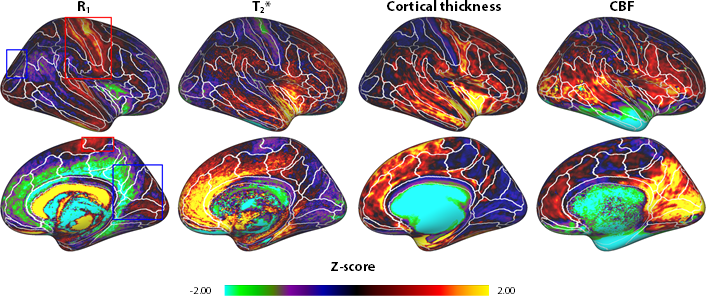
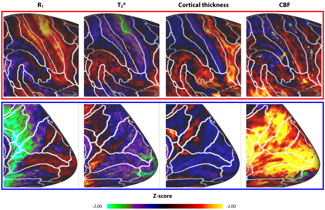
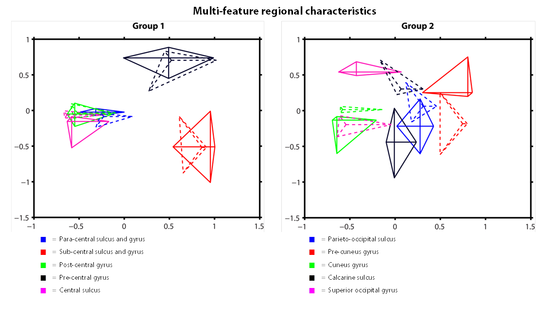
R₁ and T₂* cortical surface maps reveal a comparable pattern, as both are dominantly affected by the higher intra-cortical myelination of the primary areas (e.g. post-central gyrus, see red box in Figs. 1 and 2). Compared to these myelin-related maps, the cortical thickness map shows a different pattern, as e.g. illustrated by the difference in cortical thickness between the pre- and post-central gyri. The CBF data with smaller brain coverage (± 80%) exhibits a spatial pattern different from R₁, T₂* and cortical thickness, e.g. higher perfusion can be clearly observed in the occipital lobe and posterior cingulate, while R₁ displays differences between these two areas. Fig. 3 illustrates the multi-feature-based differentiation among several regions (color coded) within the red (group 1) and blue (group 2) boxes of Fig. 2. The location on the 2D grid is determined by their shape (i.e. each spoke corresponds to a single feature) and visualizes the differences of MRI parameters for the various brain areas. This data clearly shows that the degree of the observed change, by including CBF information (solid vs. dashed glyphs), is different across groups of regions, i.e. group 1 vs. 2.

Discussion

Here, we show the first application of multi-feature characterization of brain regions that includes CBF information, based on pre-defined regions. However, since CBF is closely coupled to brain metabolism⁶, a data-driven parcellation of brain regions that incorporates perfusion information will presumably enhance subsequent functional analysis. We can demonstrate that the CBF data is not redundant with the other quantitative MRI parameters. Therefore, we are currently setting up a fully automatic single-subject cortical parcellation routine based on hierarchical clustering that is driven by multiple parameters, which can be weighted differently to enhance clustering performance^7,8.

Acknowledgements

The authors are indebted to Prof. Dr. Andrew Webb (Leiden University Medical Centre, Leiden, Netherlands) and Dr. José Marques (Donders Institute for Brain, Cognition and Behaviour, Nijmegen, Netherlands) for providing the dielectric pads and the MATLAB code to perform the post-hoc T1 correction used in this study, respectively.