0338
Analysis of 4D flow hemodynamics parameters in BAV patients using a finite element method1Biomedical Imaging Center, Pontificia Universidad Católica de Chile, Santiago, Chile, 2Department of Electrical Engineering, Pontificia Universidad Católica de Chile, Santiago, Chile, 3Department of Cardiology, Hospital Universitari Vall d´Hebron. Vall d´Hebron Institut de Recerca (VHIR). Universitat Autònoma de Barcelona., Barcelona, Spain, 4Department of Structural and Geotechnical Engineering, Pontificia Universidad Católica de Chile, Santiago, Chile, 5Department of Radiology, School of Medicine, Pontificia Universidad Católica de Chile, Santiago, Chile
Synopsis
Bicuspid aortic valve (BAV) is one the most common cardiac defect. The progression of the defect can vary with the time and may lead to ventricular dysfunction, heart failure and death of the patient. In this work we proposed a method to obtain several hemodynamics parameters including WSS, OSI, vorticity, helicity density, viscous dissipation, energy loss and kinetic energy from 4D-flow data sets of BAV patients and healthy volunteers using a finite-element approach. We found that the viscous dissipation, helicity density, vorticity, WSS and energy loss are the most relevant hemodynamics parameters in the ascending aorta of those patients.
Purpose
Bicuspid-aortic-valve (BAV) is the most common congenital defect1. The progression of the defect can vary with the time, and the typical manifestation related with the function of the aorta are aneurysm, dissection and other complications. Recent studies in patient with BAV found that these patients exhibit altered blood flow in the ascending aorta1-4. These alterations of the blood flow may lead to changes in hemodynamics parameters including wall shear stress (WSS), oscillatory shear index (OSI), vorticity, helicity density, viscous dissipation, energy loss and kinetic energy2,5-8. Some of these proposed method to calculate the hemodynamics parameters have been using finite-differences, however, this technique cannot handle the smooth and complex boundaries of vessels in the cardiovascular system, and therefore induces important errors when the geometry is simplified9. We propose a single methodology based on finite-element analysis to obtain several 3D quantitative maps of WSS, OSI, vorticity, helicity density, viscous dissipation, energy loss and kinetic energy from a single 4D-flow data set. We show the applicability of the proposed method in healthy volunteers and in patients with BAV.Methods
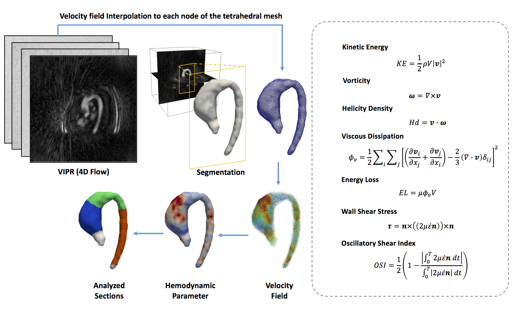
We developed a finite-element based computational framework to obtain 3D maps of different hemodynamic parameters from 4D-flow MR data as described in figure1. The algorithm is based in a similar least-squares projection method previously published10. A total of 10 healthy volunteer (age 50±15.2years, weight 78±10.7kg, height 169.2±7.9cm) and 10 patients with BAV (age 41.8±9years, weight 67.3±13.9kg, height 164.4±10.2cm) were analyzed. 4D-flow data was acquired at Hospital Universitari Vall d´Hebron in a GE 1.5T MR Scanner using the Vastly undersampled Isotropic Projection Reconstruction (VIPR) technique11. The data was acquired with a voxel resolution of 2.5x2.5x2.5mm and 39.5±6.3 cardiac phases for the group of volunteers, 34.5±3.1 cardiac phases for the group of patients. The process for creating the tetrahedral mesh is summarized in figure1. The tetrahedral mesh was generated using the Matlab available toolbox iso2mesh. The finite-element analysis was developed using the Python software, and for the visualization we used the software Paraview. Three different section were analyzed for each volunteer and patient, ascending aorta (AAo), aortic arch (AArc) and descending aorta (DAo) (see figure1). In all these section we analyze the mean, maximum and minimum values to found differences between volunteer and patient data. As statistical analysis we performed a Wilcoxon signed rank test for each parameter between volunteer and patients.Result
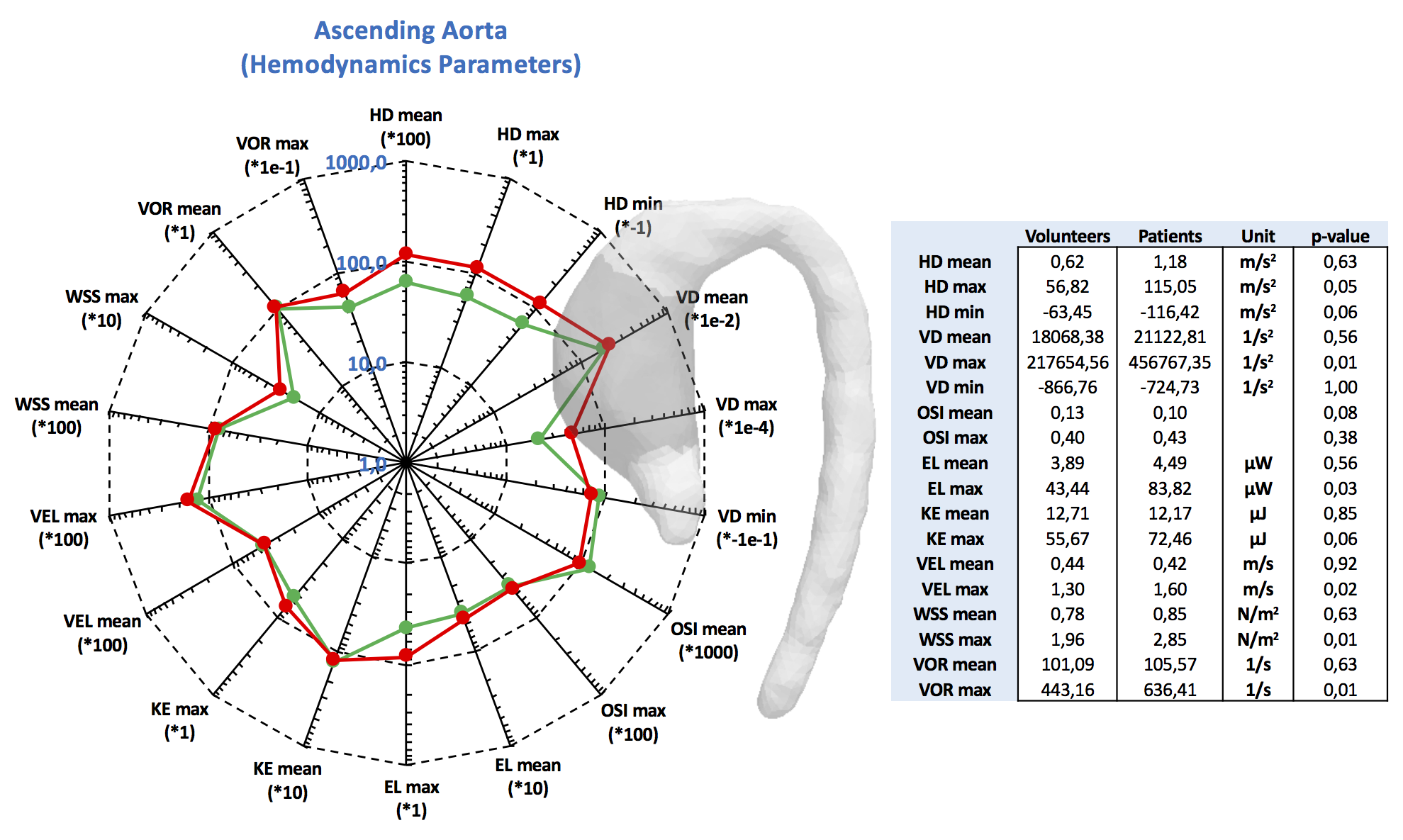
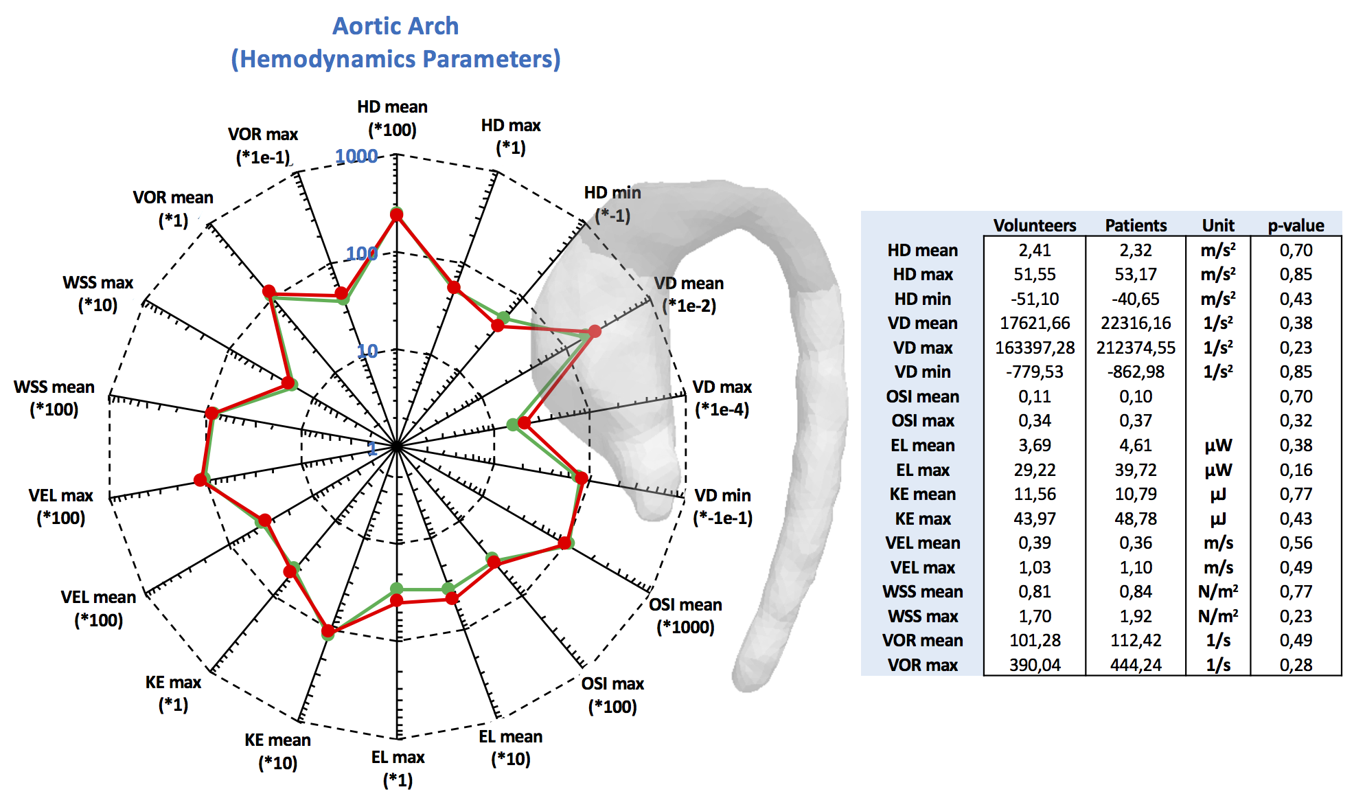
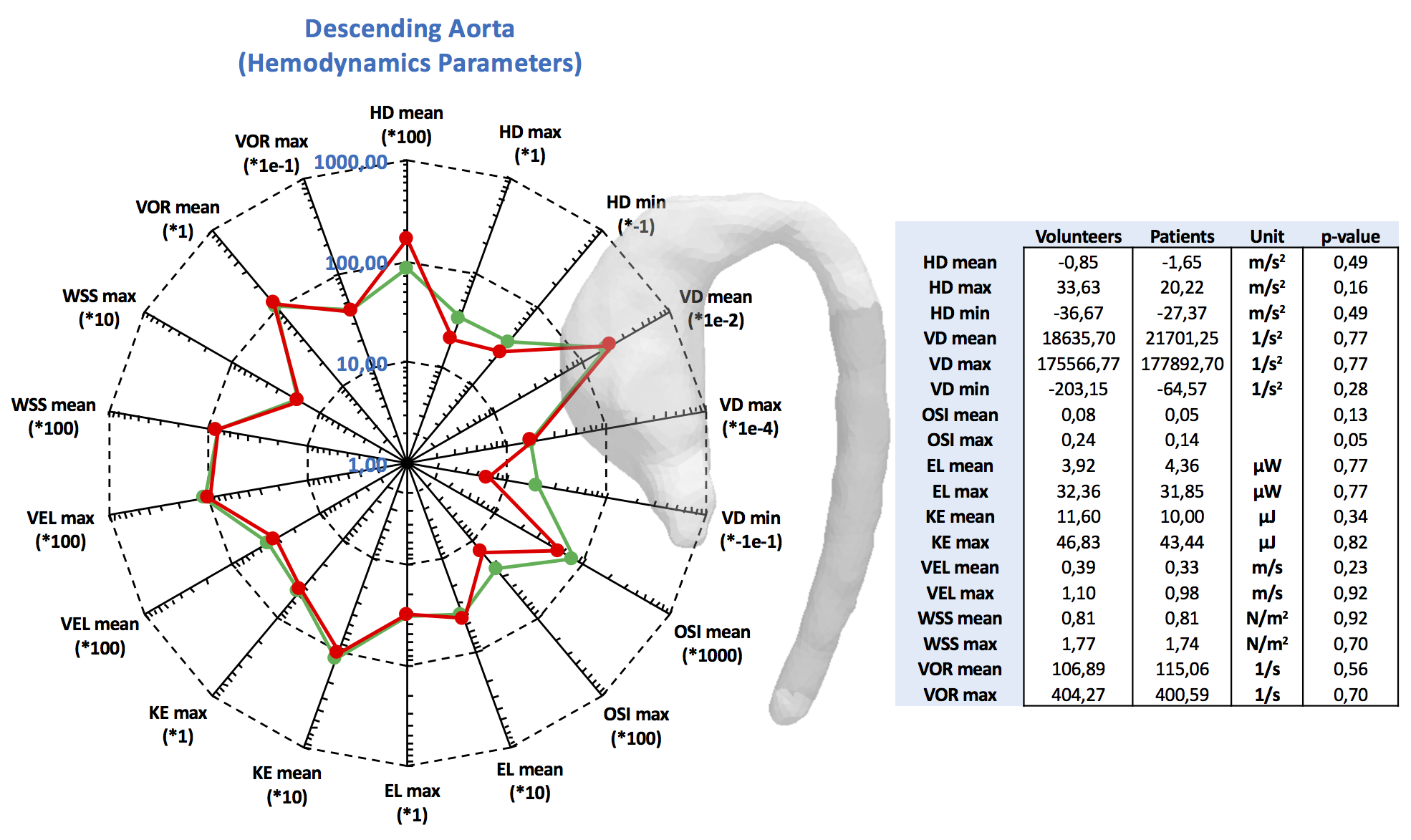
The figures 2 to 4 show the result of the analysis of the different hemodynamics parameters between volunteers (green-line) and patients (red-line). In the tables of figures 2 to 4 we show the values of hemodynamics parameters calculated in each section, and the p-value obtained by the Wilcoxon signed rank test (p≤0.05 was considered statistically significant). We observed that the AAo section shows the largest differences of hemodynamics parameters between volunteer and patient data (Figure2). The Wilcoxon signed rank test show that there were significant differences for the following variables: helicity density max, viscous dissipation max, energy loss max, velocity max, WSS max and vorticity max. Similar finding has been previously reported2,5-8. There were not significant differences between the group of volunteer and patients in the AArc and in the DAo (Figure3 and 4).
In figure5, we show 3D maps of different hemodynamics parameters for one representative volunteer and one patient to illustrate the differences between both groups. In the patient there is an eccentricity in the blood flow ejected by the left ventricle at systole (see velocity data), generating a jet that collides in the right side of the ascending aorta, possibly resulting in the dilatation of the vessel in this section. This process induces an increment of some hemodynamic parameters in this region.
Discussion and Conclusion
We have presented a method that allowed us to obtain several 3D maps of different hemodynamic parameters derive from a single 4D-flow data sets using a finite-element method. The great advantage of the proposed approach is that pre-processing of the data, including segmentations and mesh creation, is performed only once, but several quantitative hemodynamic parameters can be obtained simultaneously. This method provides hemodynamic data that can be used to identify which parameters are more sensitive to a particular disease, and also to identify which areas are being more affected. From the analysis of the data, we can conclude that only the ascending aorta showed significant different hemodynamics between volunteer and BAV patients. In particular, we found that viscous dissipation, helicity density, vorticity, WSS and energy loss showed statistical differences between both groups.Acknowledgements
Thank to grant, CONICYT - PIA - Anillo ACT1416, CONICYT FONDEF/I Concurso IDeA en dos etapas ID15|10284, and FONDECYT #1141036. Sotelo J. Thanks to the School of Engineering, Pontificia Universidad Católica de Chile, for his Post-Doctoral Fellow. Guala A. has received funding from the European Union Seventh Framework Programme FP7/People under grant agreement n° 267128.References
1. Siu SC, Silversides CK. Bicuspid aortic valve disease. J Am Coll Cardiol. 2010 Jun 22;55(25):2789-800.
2. Allen BD, van Ooij P, Barker AJ, et al. Thoracic aorta 3D hemodynamics in pediatric and young adult patients with bicuspid aortic valve. J Magn Reson Imaging. 2015 Oct;42(4):954-63.
3. Hope MD, Hope TA, Meadows AK, et al. Bicuspid aortic valve: four-dimensional MR evaluation of ascending aortic systolic flow patterns. Radiology 2010;255:53–61. ?
4. Bissell MM, Hess AT, Biasiolli L, et al. Aortic dilation in bicuspid aortic valve disease: flow pattern is a major contributor and differs with valve fusion type. Circ Cardiovasc Imaging 2013;6:499–507. ?
5. Saikrishnan N, Mirabella L, Yoganathan AP. Bicuspid aortic valves are associated with increased wall and turbulence shear stress levels compared to trileaflet aortic valves. Biomech Model Mechanobiol. 2015 Jun;14(3):577-88.
6. Barker AJ, van Ooij P, Bandi K, et al. Viscous energy loss in the presence of abnormal aortic flow. Magn Reson Med. 2014 Sep;72(3):620-8.
7. Binter C, Gülan U, Holzner M, Kozerke S. On the accuracy of viscous and turbulent loss quantification in stenotic aortic flow using phase-contrast MRI. Magn Reson Med. 2016 Jul;76(1):191-6.
8. van Ooij P, Garcia J, Potters WV, et al. Age-related changes in aortic 3D blood flow velocities and wall shear stress: Implications for the identification of altered hemodynamics in patients with aortic valve disease. J Magn Reson Imaging. 2016 May;43(5):1239-49.
9. Zienkiewicz OC, Taylor RL, Zhu JZ. The finite element method: Its basis and fundamentals, sixth ed. London: Butterworth-Heinemann. 2005.
10. Sotelo J, Urbina J, Valverde I, et al. 3D Quantification of Wall Shear Stress and Oscillatory Shear Index Using a Finite-Element Method in 3D CINE PC-MRI Data of the Thoracic Aorta. IEEE Trans Med Imaging. 2016 Jun;35(6):1475-87.
11. Barger AV, Block WF, Toropov Y, et al. Time-resolved contrast-enhanced imaging with isotropic resolution and broad coverage using an undersampled 3D projection trajectory. Magn Reson Med. 2002 Aug;48(2):297-305.
Figures