0240
Global signal regression alters the correlation between resting-state BOLD fluctuations and EEG vigilance measuresMaryam Falahpour1, Alican Nalci1, Chi Wah Wong1, and Thomas Liu1
1Center for functional MRI, University of California San Diego, San Diego, CA, United States
Synopsis
Global signal regression (GSR) is a commonly used preprocessing approach in the analysis of resting state fMRI data. Utilizing simultaneously acquired EEG/fMRI data in humans, we found that GSR alters the correlation between the resting-state BOLD fluctuations and EEG vigilance. We show that GSR reveals BOLD-EEG correlations that are otherwise obscured and use a time segmentation approach to argue that the observed effects are not simply an artifact of GSR.
Purpose
Global signal regression (GSR) is a commonly used albeit controversial preprocessing approach in the analysis of resting state fMRI data.1 However, there is also growing evidence for the existence of a significant neural component in the global signal2, suggesting that GSR could potentially remove valuable information. Utilizing simultaneously acquired EEG/fMRI data in humans, we examined the effect of GSR on the correlation between resting-state BOLD fluctuations and EEG vigilance measures. We show that GSR reveals correlations that are otherwise obscured and use a time segmentation approach to argue that the observed effects are not simply an artifact of GSR.Methods
EEG-fMRI data were simultaneously acquired on 9 healthy subjects during three eyes-closed resting-state sessions using a 3T GE MR750 system and a 64 channel EEG system (Brain Products). BOLD fMRI data were acquired with echo planar imaging with 166 volumes, 3.4×3.4×5mm3 voxel size, 64×64 matrix size, TR=1.8s, TE=30ms. Preprocessing steps are described in.2 Vigilance was defined as the average alpha amplitude (7-13Hz) divided by the average amplitude in the delta and theta (1-7Hz) bands,2 and the resulting time course was convolved with a hemodynamic response function. The global signal (GS) was formed by averaging the percent change BOLD time series across all brain voxels. For each run, the temporal correlation between EEG vigilance and BOLD time courses was calculated before and after GSR. Additionally, we split the time points into two subsets. The first set contained only time points where the GS magnitude was either high (above the third quartile (Q3)) or low (below the first quartile (Q1)). The second set contained points in the interquartile range (IQR: middle 50%). Correlations between the vigilance and BOLD time courses were computed on each set separately (without GSR). For each processing approach, a one sample t-test (3dttest++ from AFNI with t-test randomization to minimize the FPR) was performed on the Fisher-z transformed correlation maps.Results
Figure 1 shows group result z-score maps (from 3dttest++) for each condition. Consistent with prior studies,3-4 we found significant positive BOLD-vigilance correlations in the thalamus and negative correlations in widespread regions of the brain, including the posterior cingulate, cuneus, precuneus, lingual gyrus, and insula. After GSR, there was a significant reduction in the magnitude and the extent of the negative correlations, whereas the extent of the positive correlations in sub-regions of the cingulate gyrus increased. See Figures 1A and 1B. We examined the individual correlations (as z-values) averaged within three ROIs showing significant BOLD-vigilance correlations. Figure 2A shows that there was a significant increase in the z-values (indicative of an increase in correlation between EEG and BOLD) with GSR (as compared to no GSR) in ROI1 (anterior and middle cingulate gyrus) and ROI3 (lingual gyrus, calcarine gyrus, cuneus) but no significant difference in ROI2 (thalamus). Figure 3 displays the GS time series from a representative subject. The high/low value points are marked with red crosses, while the points in the interquartile range are marked with black circles. The spatial pattern of significant BOLD-vigilance correlations obtained when using the high/low subset (Figure 1C) is similar to that found for the original data (all time points) in Figure 1A. The pattern of correlations obtained when using the interquartile range (Figure 1D) is similar to that found after GSR (Figure 1B). In addition, the relationship between the z-values for the correlations from the interquartile and high/low subsets (Figure 2B) is similar to that found when comparing the correlations obtained with GSR and no GSR (Figure 2A).Discussion
We have shown that GSR alters the correlation between BOLD fluctuations and EEG vigilance. The correlations obtained with GSR are similar to those obtained when using time points in the interquartile range, suggesting that GSR may help to reveal correlations in time segments where the GS magnitude is low. It is important to note that the positive correlations observed in the anterior and middle cingulate gyrus (Fig. 1B and 1D) are not readily observed in the original data (Fig 1A). The similarity of the results obtained with the original data and the high/low subset suggests that the original correlations are dominated by data from the high/low subset making it difficult to observe the BOLD-EEG coupling in the interquartile subset. Furthermore, because the correlations in the cingulate gyrus can be observed in data from the inter-quartile subset (without GSR), it is unlikely that they are simply an artifact of GSR. Our findings suggest that GSR and time-segmentation approaches may be useful for uncovering relations between BOLD and vigilance that might not be detectable with conventional approaches.Acknowledgements
No acknowledgement found.References
[1] Murphy et. al., Neuroimage 2009, 44:893-905.
[2] Wong et. al., Neuroimage 2013, 83:983-990.
[3] Goldman et. al.. Neuroreport 2002, 13: 2487-2492
[4] Liu et. al., Neuroimage 2012, 63:1060-1069.
Figures
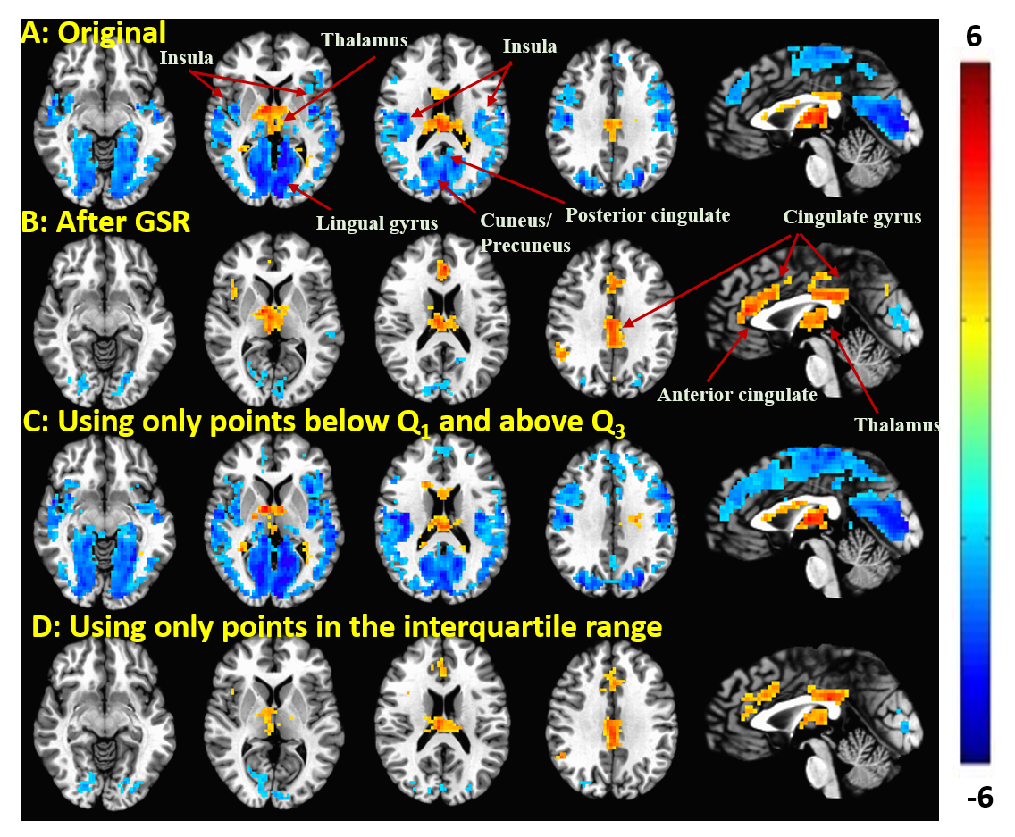
Figure 1. Group result z-scores (from 3ttest++) showing areas of
significant correlation between the BOLD data and EEG vigilance when using: A: Original data (before GSR); B: Data after
GSR; C: Data from points below the first and above the third quartile (e.g. marked
with red ”x” in Figure 3) of the GS time series; D: Data from points in the
interquartile range (e.g. marked with black ”o” in Figure 3) of the GS. Maps are thresholded at p<0.05 (corrected).
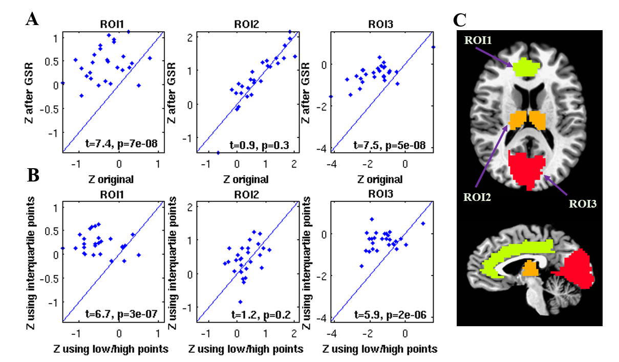
Figure 2. A: Average z-values from each ROI obtained after GSR
plotted versus the corresponding values obtained prior to GSR (original data). B: Average z-values from each ROI derived from
interquartile points plotted against the corresponding values from low/high
value points. C: 3 ROIs defined from an anatomical parcellation (AFNI TT_caez_ml_18)
based on overlap with clusters showing significant correlations. ROI1 includes
left and right anterior cingulate and middle cingulate gyrus. ROI2 includes left and right thalamus. ROI3
includes left and right lingual gyrus, calcarine gyrus, and cuneus.
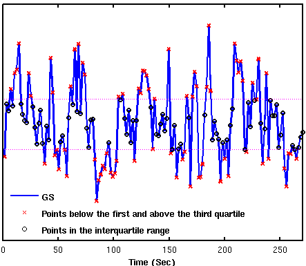
Figure 3. Global signal time series from a representative subject.
Data points were divided into 2 subsets. The first set contains the points
below the first quartile and above the third quartile (Q1 and
Q3, dashed purple lines)
of the GS time series (marked with red “x“). The second set contains the points
in the interquartile range (marked with black “o”).