Synopsis

The high frequency networks are hard to be observed with standard fMRI data. Those networks were submerged in the non-BOLD signal and could not be observed with standard fMRI methods. In this work, Multiband Multi-echo (MBME) sequence is used to sample brain fluctuations in high frequency (TR=0.75).By using acquired 8 echoes, T2* and I0 (initial intensity) values are calculated and fluctuations in the brain were separated into BOLD and non-BOLD. Results showed that there is an improved detection in several high frequency networks like LECN, dDMN, Language and high Visual networks by using the separated BOLD signal.

Introduction:

Methods:

Imaging: Two healthy volunteers asked to rest during scan, eight-echo Multiband Multi-echo sequence is used on Siemens MAGNETOM Prisma 3.0T scanner with a 64 channel head coil. And the experiment parameters are TEs = [7.8, 20.65, 33.5, 46.35, 59.2, 72.05, 84.9, 97.75], TR=0.75ms, 3*3*4.4 mm3, 25% slice gap, 24 slices, SMS factor = 4, partial Fourier = 7/8, Grappa Acceleration factor = 2.

As the MRI signal has an exponential decay$$$S=I_0exp(-TE/T_2^*)$$$, $$$I_0$$$ and $$$T2*$$$ value were got for each TR by nonlinear fitting the exponential curve for each voxel with least-square limitation. Based on $$$I_0$$$ and $$$T2*$$$ time series, we can achieve the signal contribution from both $$$I_0$$$ and $$$T2*$$$ side. Signal variation could be formulized as follows,$$S=S_0+S_{T_2^*}+S_{I_0}$$

and could be expand by Taylor expansion as follows;

$$S(I_0,T_2^*)=S(\overline{I_0},\overline{T_2^*})+\frac{\partial S\cdot\triangle T_2^*}{\partial T_2^*}+\frac{\partial S\cdot\triangle I_0}{\partial I_0}+O({\triangle I_0}^2,{\triangle T_2^*}^2)$$

where;

$$$S$$$ is the original fMRI data at the 3rd echo with the TE = 33.5 ms,

$$$S_0$$$ is the constant mean value of the fMRI data, which reflect the base line of the functional data,

$$$S_{T_2^*}$$$ is the signal variation caused by T2* fluctuation, which can also be called BOLD signal,

$$$S_{I_0}$$$ is the signal variation caused by the $$$I_0$$$ changes, which can be called non-BOLD signal.

Pre-processing: The preprocessing of S, $$$S_{T_2^*}$$$ time-courses included motion correction, registration to MNI atlas, spatial smoothing using a 7 mm FWHM Gaussian filter and temporal band-pass filtering (0.01 to 0.1 Hz) and (0.1 to 0.25 Hz) .

Seed-based functional connectivity map : First functional images were registered to standard MNI space, center points of functional atlas (5) were selected as a seed point. Seed based connectivity is calculated for both BOLD signal ($$$S_{T_2^*}$$$) and unseparated signal ($$$S$$$) under two frequency bands.

Results & Discussion:

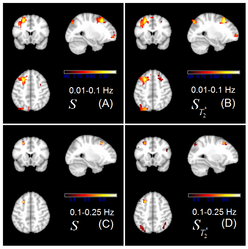
The functional networks were observed for both BOLD signal ($$$S_{T_2^*}$$$) and unseparated signal ($$$S$$$) under low frequency. At low frequencies network pattern came out quite similar between $$$S_{T_2^*}$$$ and S as it is shown in Figure 1 (A) and (B). For higher frequency the distant connectivity could be more visible observed in $$$S_{T_2^*}$$$ , but could hardly be observed in Figure 1(C) and (D) with the same threshold.

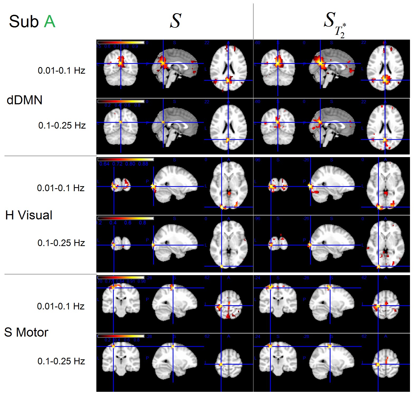
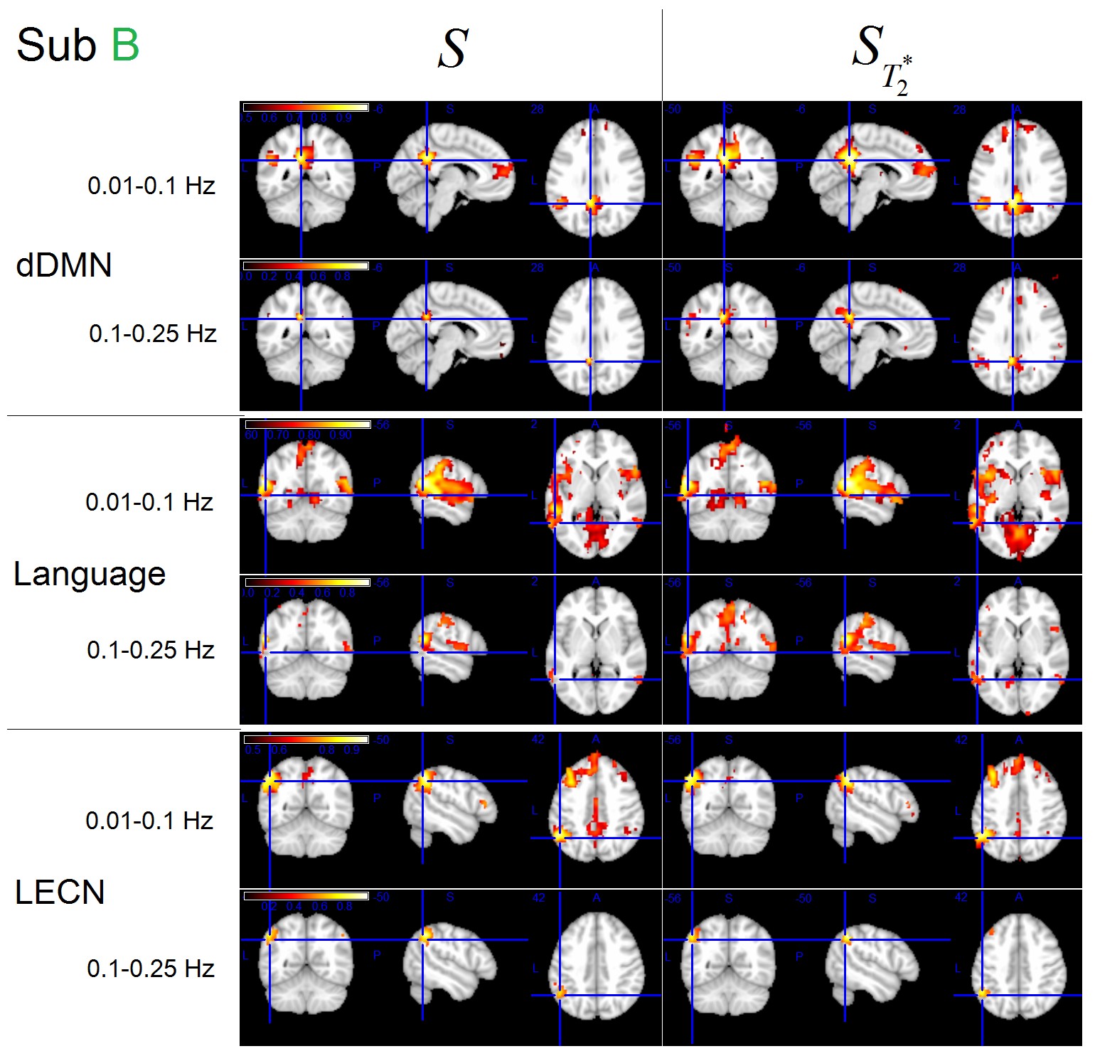
The effects were only observed for some networks of our two volunteers and the results are shown respectively. Figure 2 shows the dorsal DMN, High Visual network and sensorimotor network connectivity for subject A. Figure 3 shows the dorsal DMN, Language and LECN network connectivity for subject B.

In the functional connectivity map, a high threshold was used for low frequency network and a low threshold was used for high frequency network.

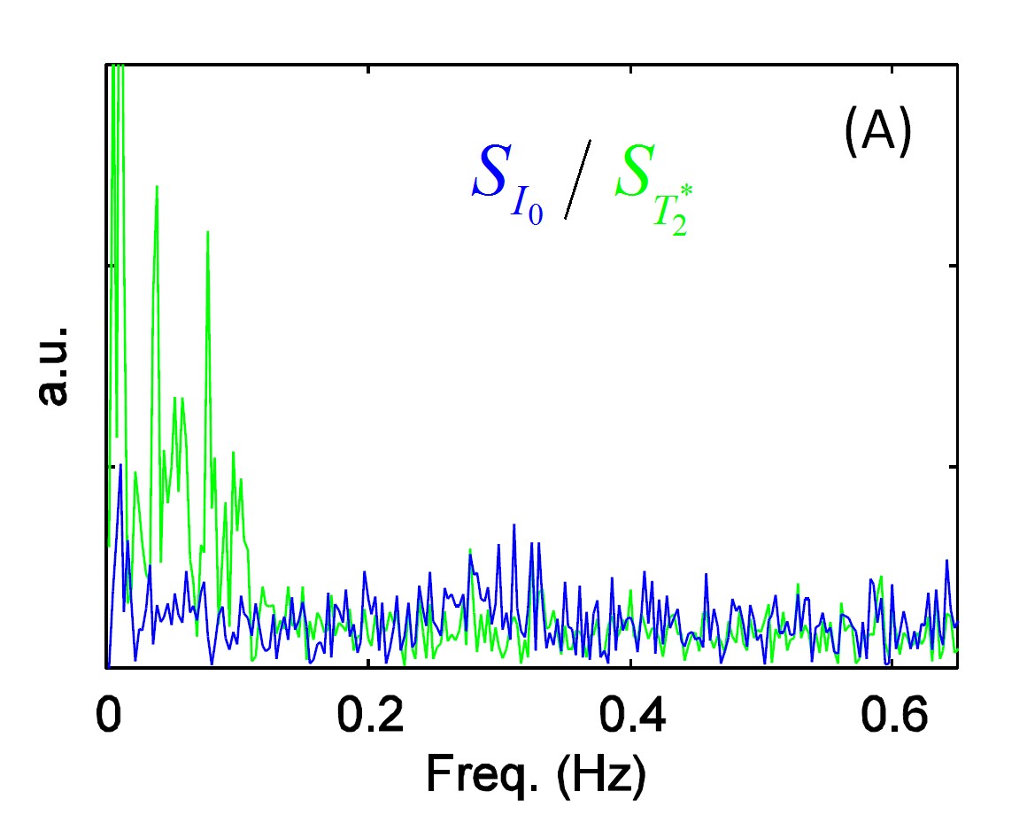
The $$$S$$$ makeup $$$S_{I_0}$$$ and $$$S_{T_2^*}$$$ are shown in spectrum in Figure 4. In the low frequency bands the power BOLD signal is larger than non-BOLD signal. In higher frequency the power of both signals are almost the same. This shows the reason that the network in high frequency is hard to be detected only with the help of separated $$$S_{T_2^*}$$$.

Conclusion:

Acknowledgements

References

1. Lee H L, Zahneisen B, Hugger T, et al. Tracking dynamic resting-state networks at higher frequencies using MR-encephalography[J]. Neuroimage, 2013, 65: 216-222.

2. Smith-Collins A P R, Luyt K, Heep A, et al. High frequency functional brain networks in neonates revealed by rapid acquisition resting state fMRI[J]. Human brain mapping, 2015, 36(7): 2483-2494.

3. Speck O, Hennig J. Functional Imaging by I0-and T2*-parameter mapping using multi-image EPI[J]. Magnetic resonance in medicine, 1998, 40(2): 243-248.

4. Kundu, Prantik, et al. "Differentiating BOLD and non-BOLD signals in fMRI time series using multi-echo EPI." Neuroimage 60.3 (2012): 1759-1770.

5. Shirer WR, Ryali S, Rykhlevskaia E, Menon V, Greicius MD: Decoding subject-driven cognitive states with whole-brain connectivity patterns. Cereb Cortex (2012)