0128
Quantification of Flow by Magnetic Resonance Fingerprinting1Medical Physics in Radiology, German Cancer Research Center (DKFZ), Heidelberg, Germany, 2Institute for Forensic Medicine and Traffic Medicine, Germany, 3Physikalisch-Technische Bundesanstalt (PTB), Braunschweig and Berlin, Germany
Synopsis
The goal of this work is to investigate and demonstrate 'flow MRF', a technique that quantifies T1 and T2 within static tissue regions around a vessel (e.g. vessel wall) with high spatial resolution while simultaneously quantifying the 3D blood velocity vector within the vessel with high precision and high spatiotemporal resolution. The results show that simultaneous mapping of pulsatile flow and T1/T2 quantification of static tissue is feasible with MRF. The quantification of flow as an additional parameter will further increase the efficiency of MRF and may provide new diagnostic value in cardiovascular diseases.
Purpose
Magnetic Resonance Fingerprinting (MRF) has been shown to be a fast and accurate technique to quantify tissue parameters such as T1, T2, B0 and others [1]. However, conventional MRF relies on the target tissues to be static; temporally varying functional parameters, such as pulsatile flow, are challenging to quantify. The goal of this work is to investigate and demonstrate 'flow MRF', a technique that quantifies T1 and T2 within static tissue regions around a vessel (e.g. vessel wall) with high spatial resolution while simultaneously quantifying the 3D blood velocity vector within the vessel with high precision and high spatiotemporal resolution. The concept is demonstrated in phantoms with pulsative flow at ultra-high field.Background
MRF uses spatially undersampled acquisitions in combination with temporally varying sequence parameters such as TR, TE, flip angle (FA) and others, to create unique signal evolutions ('fingerprints') of each tissue type. By matching the signal evolutions to a dictionary with simulated fingerprints, relaxation parameters such as T1 and T2 can be reconstructed. While spatial undersampling artifacts have limited influence on the quantification because they appear noise-like in time, the quantification of functional parameters is challenging because both signal variations occur in the temporal domain.
Blood flow is typically quantified by two or multiple phase contrast cine acquisitions with varying bipolar velocity encoding gradients with defined first gradient moments $$$m_1=\int{G(t)}\cdot t\,dt$$$. The velocity is proportional to the phase difference and the maximum encoding velocity (VENC) is controlled via m1.
Method
A standard FISP MRF sequence pattern [2], consisting of an initial inversion pulse followed by an acquisition train with variable TR and FA, was modified to have constant TR/TE of 9.21ms/5.01ms (Fig.1) and the spiral readout was replaced by a radial center-out trajectory. This generates a constant signal phase throughout the acquisition train, except for an initial period (a few TRs) after the slice-selective adiabatic inversion. By including bipolar flow-encoding gradients with varying $$$m_1$$$ but $$$m_0 = \int{G(t)}\,dt = 0$$$, quantification of blood flow within the vessel is decoupled from parameter determination of the surrounding tissue: only the velocities are encoded in the signal phase. The encoding of T1 and T2 in the static tissue, however, is unperturbed by the flow-encoding scheme.
m1 of the bipolar gradients is varied pseudo randomly between $$$0$$$ and $$$50\frac{mT}{m}\cdot{ms}^2$$$ (minimum $$$VENC=23cm/s$$$) on all three gradient axes (Fig.2). The acquisition train in Fig.1a was obtained 11 times with different k-space projections, separated by 8s waiting periods prior to the next inversion. Total measurement time was 3min per slice. Imaging was performed in axial orientation in a cylindrical flow phantom consisting of 4 pipes with different diameters of 4.2/7.8/12.1/15.5mm; the 2 largest pipes were connected to a flow pump (Shelly Medical Imaging Technologies, CardioFlow 5000 MR), generating a pulsatile pattern. Velocity data was binned into 36 cardiac phases that were separately reconstructed, while no binning was performed for static tissue parameter determination. Bloch-Siegert based B1 maps were included in the reconstruction to improve determination of T2. Measurements were performed on a Magnetom 7T (Siemens, Germany) using a 24-channel head coil (Nova Medical Inc., USA).
Results
The animated Fig.3 illustrates a magnitude image of the flow phantom with an overlay of velocity values obtained by flow MRF within the two pipes with flow. The corresponding plot displays resulting flow velocities averaged within the ROI (black box in Fig.3) for flow MRF as well as for a 2D-cine phase contrast based method with 3D velocity encoding (acquisition time: 2:10min). A maximum deviation of 5cm/s between flow MRF and the reference was observed.
Figure 4 shows parameter maps of T1 and T2 in therelaxometric phantom alongside established reference methods. Figure 5 displays the correlation of the MRF with the spin-echo based reference method. A deviation of 3% for T1 and 12% for T2 can be noted.
Discussion
The results of this study demonstrate that simultaneous mapping of pulsatile flow and T1/T2 quantification of static tissue is feasible with MRF. Including variable m1 with peak values of $$$50\frac{mT}{m}\cdot{ms}^2$$$ allows high velocity sensitivity without typical phase aliasing, a common issue in standard flow imaging. The current implementation relies on a regular flow pattern, which might not always be assumable in a patient. The combination of MRF and retrospective binning is feasible and under current investigation. Optimizing the FA pattern to allow for the simultaneous quantification of B1 will further increase the precision of the T1 and T2 maps. The quantification of flow as an additional parameter will further increase the efficiency of MRF and may provide new diagnostic value in cardiovascular diseases.Acknowledgements
No acknowledgement found.References
[1] Ma D, Gulani V, Seiberlich N, Liu K, Sunshine JL, Duerk JL, Griswold MA. Magnetic Resonance Fingerprinting. Nature 495, 187–192.
[2] Jiang Y, Ma D, Seiberlich N, Gulani V, Griswold MA. MR fingerprinting using fast imaging with steady state precession (FISP) with spiral readout. Magn. Reson. Med., 74: 1621–1631.
Figures
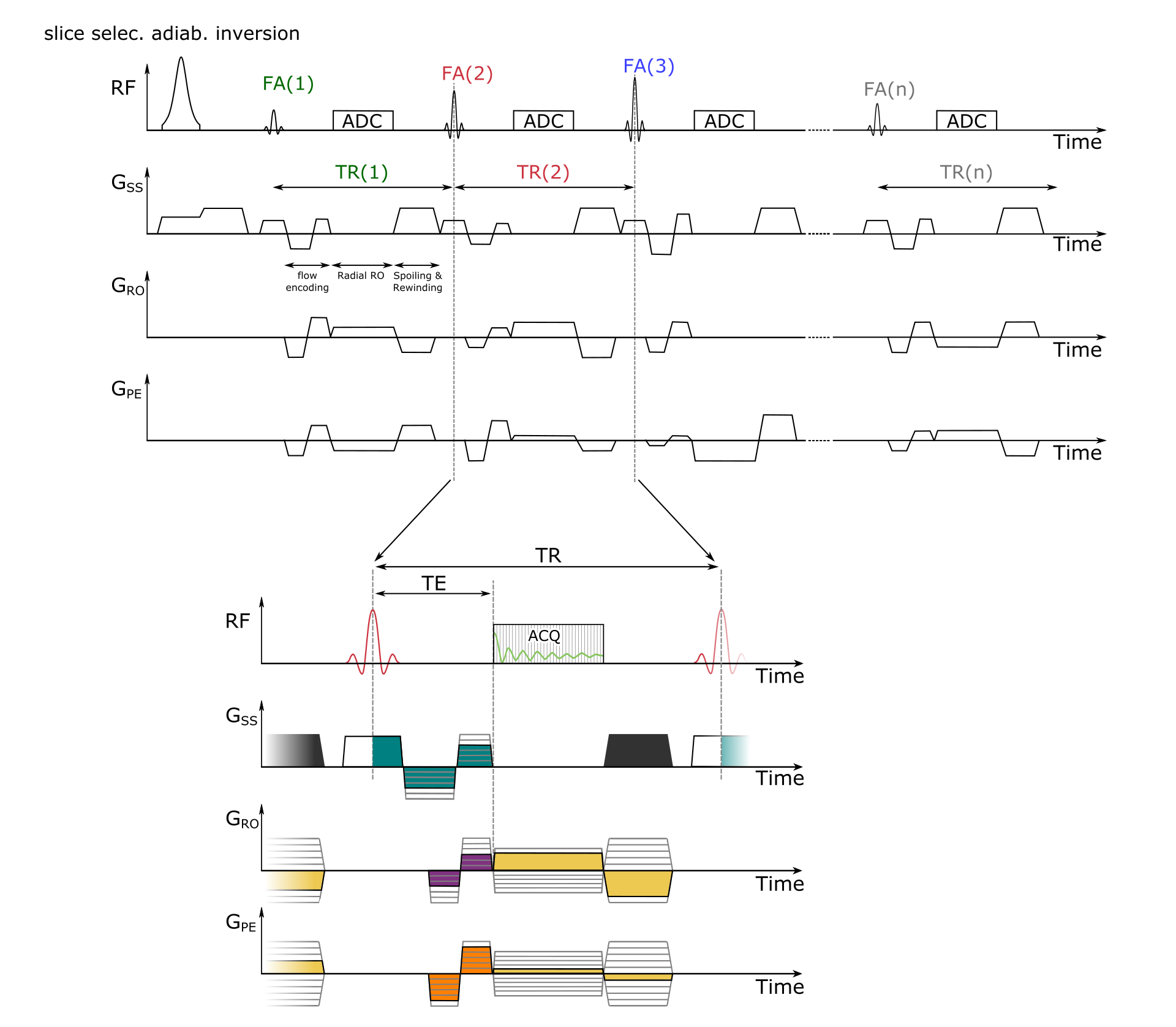
Figure 1:
Sequence diagram of the FISP-based MRF sequence with simultaneous 3D velocity quantification. The colored gradient areas are always chosen such that the zeroth order moment adds up to zero. Bipolar gradients before the radial readout (color: turquoise, purple and orange) encode the velocity and vary the first order moment pseudo randomly throughout the acquisition train. The radial center-out readout is rewound completely (color: yellow), and the magnetization is dephased by 8pi in the slice direction (grey gradient).
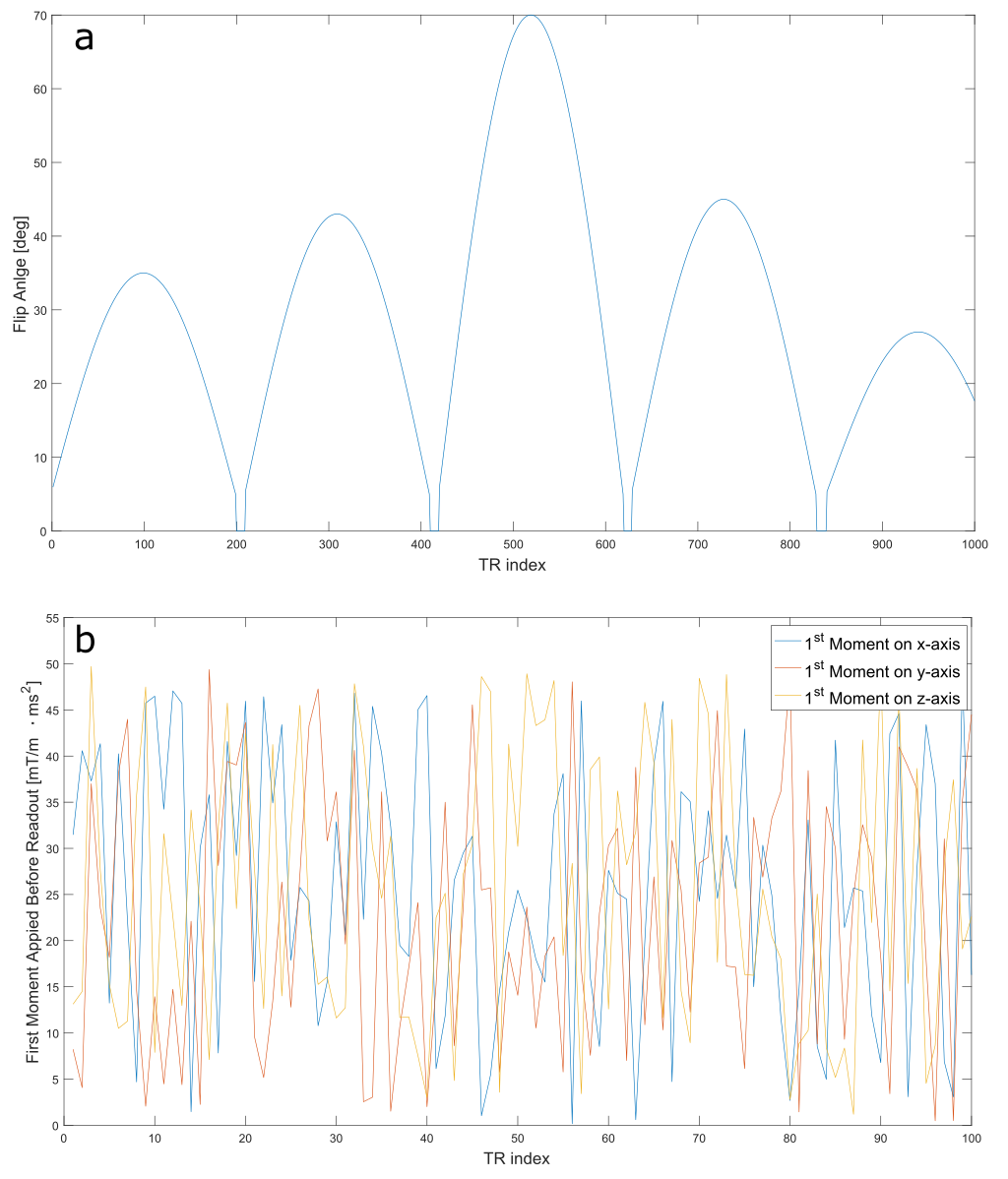
Figure 2:
In a) the complete pattern of the nominal flip angle is shown. This pattern was taken from the FISP MRF publication [2]. b) displays the pseudo random variation of the flow encoding moment for the first 100 TRs. The pattern is continued in a similar manner for the remaining 900 TR intervals of the acquisition train.
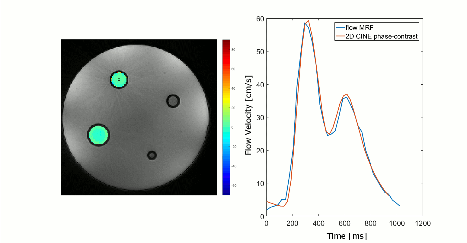
Figure 3:
The animation on the left displays an overlay of the temporal evolution of the pulsatile flow, as reconstructed by the MRF sequence, on a magnitude image of the phantom. The nominal in-plane resolution is 0.56mm and 36 flow phases where reconstructed over a period of 1024ms, resulting in a temporal resolution of 28.4ms. Only the z-component of the flow is displayed. The plot on the right displays the mean flow velocity in the ROI indicated by the black box for the flow MRF measurement and for the reference 2D CINE phase contrast based method with 3-directional velocity encoding.
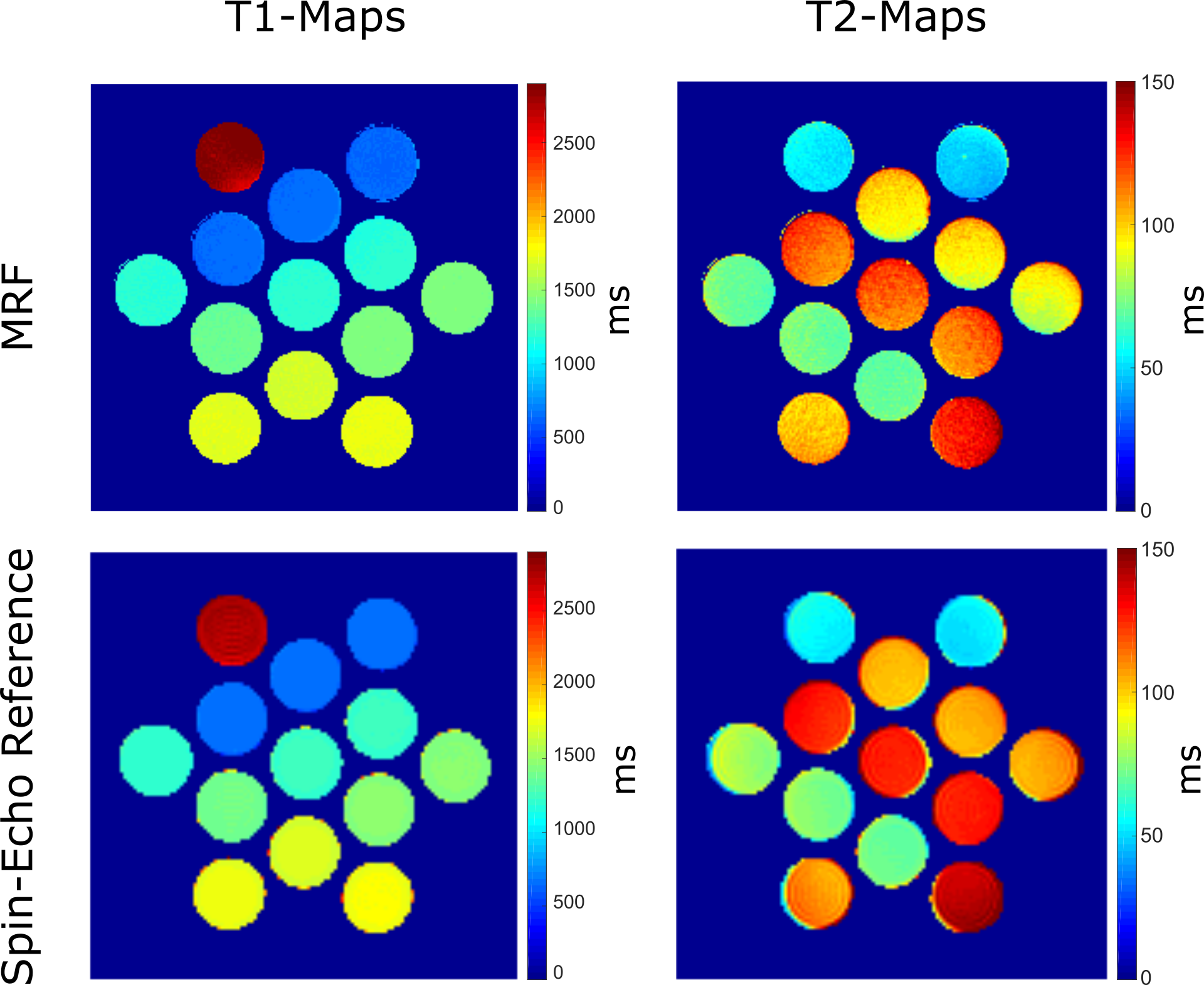
Figure 4:
Quantitative T1 and T2 maps determined by MRF and a spin-echo based reference. A standard vendor-provided spin-echo sequence was used for the determination of T2 and an inversion recovery spin-echo sequence for the determination of T1.
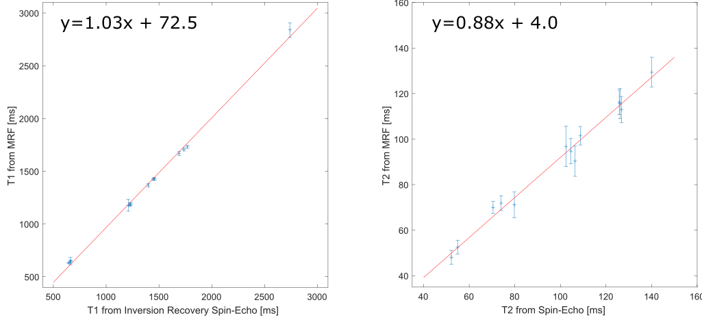
Figure 5:
Correlation between the flow MRF measurement and spin-echo based references. The distribution of relaxation times from the multi-compartment phantom was fitted by a linear model (red line).