0127
Relaxation in Polar Coordinates: Analysis and Optimization of MR-Fingerprinting1Dept. of Radiology - Bernard and Irene Schwartz Center for Biomedical Imaging, New York University School of Medicine, New York, NY, United States, 2Dept. of Radiology - Center for Advanced Imaging Innovation and Research, New York University School of Medicine, New York, NY, United States
Synopsis
This work analyses relaxation in balanced non-steady-state free precession sequences. Transforming the Bloch equation to polar coordinates gives insights in the spin dynamics and provides the basis for robust numerical optimization of the excitation pattern. The employed optimal control algorithm results in spin trajectories that allow for parameter mapping with considerably reduced noise, as shown in in vivo MR-fingerprinting experiments. The simple shapes of the optimized spin trajectories provide a basis for further analysis of the encoding process of relaxation times for parameter mapping.
Purpose
MR-Fingerprinting1 (MRF) opens a rich space for sequences design and allows to freely exploit the spin dynamics in order to encode physical parameters such as relaxation times. The first published MRF-methods use heuristically-found pattern of RF-pulses1,2,3 and more recent work aimed at numerically optimizing the sequence design4,5,6. However, these methods provide little insight in the underlying spin dynamics. Here, we analyze relaxation whith the Bloch equation in polar coordinates and simplify the model for pseudo steady-state free precession (SSFP) sequences7. This provides insight into the encoding of relaxation times and allows for robust numerical optimization.Theory
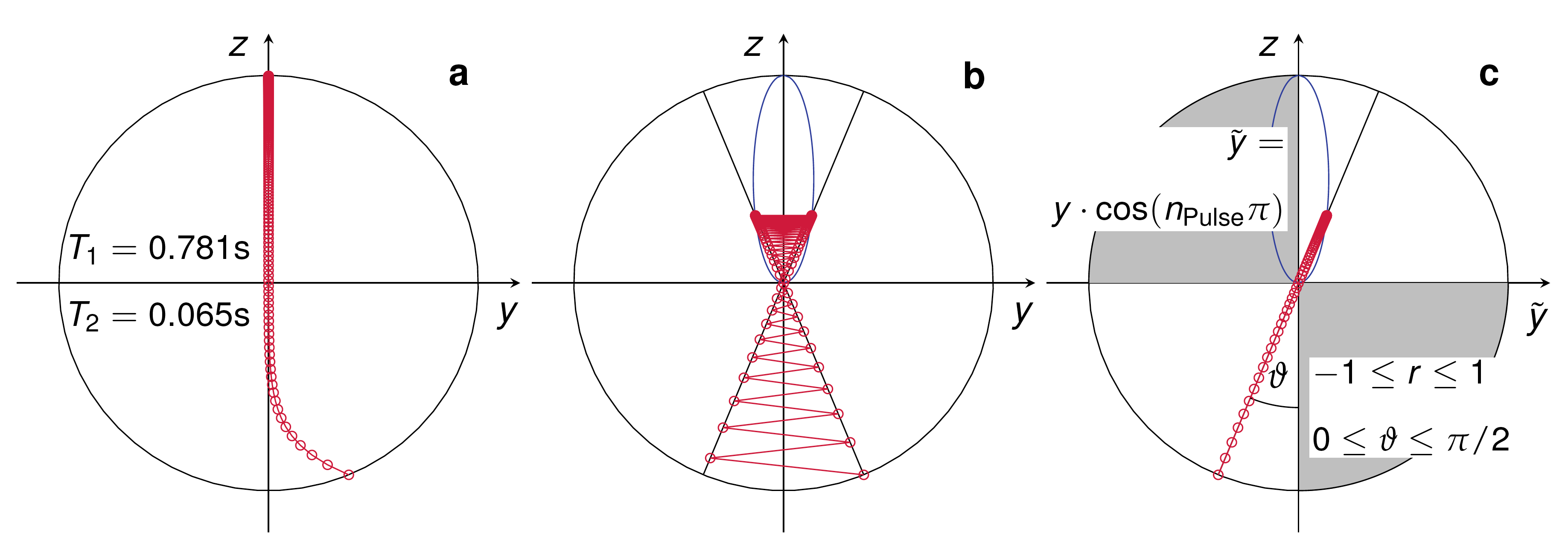
Balanced-SSFP sequences employ equidistant RF-pulses with a constant flip angle and a phase increment of $$$\pi$$$ for consecutive pulses, which refocuses all magnetization within a passband at $$$TE=TR/2$$$. This spin-echo-like property can be translated to MRF-sequences with varying flip angles7, allowing to neglect dephasing and to describe the spin dynamics by 2D Bloch-equations:$$\dot{y}(t)=\frac{y(t)}{T_2}-\omega_1(t)z(t)$$$$\dot{z}(t)=\frac{1-z(t)}{T_1}+\omega_1(t)y(t).$$Here, $$$y(t),z(t)$$$ are the transversal and longitudinal component of the magnetization, $$$\dot{y}(t),\dot{z}(t)$$$ their temporal derivatives and $$$\omega_1(t)$$$ denotes the real valued RF-pulses. The alternating RF-pulses with a constant flip angle forces the magnetization onto a cone9 (Figure$$$~$$$1b). Switching to an oscillating frame of reference with $$$\tilde{y}(t)=y(t)\cdot\cos(n\pi)\forall{n}\in\{0,\ldots,N_{\text{Pulse}}-1\}$$$, one observes relaxation purely in the radial direction (Figure$$$~$$$1c). This motivates to transform the Bloch equations to the modified polar coordinates $$$-1\leq{r(t)}\leq1,0\leq\vartheta(t)\leq\pi/2$$$ defined by $$$\tilde{y}=r\sin{\vartheta},z=r\cos{\vartheta}$$$. The radial component is given by$$\dot{r}(t)=\frac{r(t)\sin^2{\vartheta(t)}}{T_2}+\frac{\cos{\vartheta(t)}}{T_1}-\frac{r(t)\cos^2{\vartheta(t)}}{T_1}.$$For case of $$${TR}\ll\{T_1,T_2\}$$$ and smoothly varying flip angles, the orthoradial relaxation in consecutive TRs cancel each other, allowing for the approximation$$\dot{\vartheta}(t)\approx-\omega_1(t).$$Methods
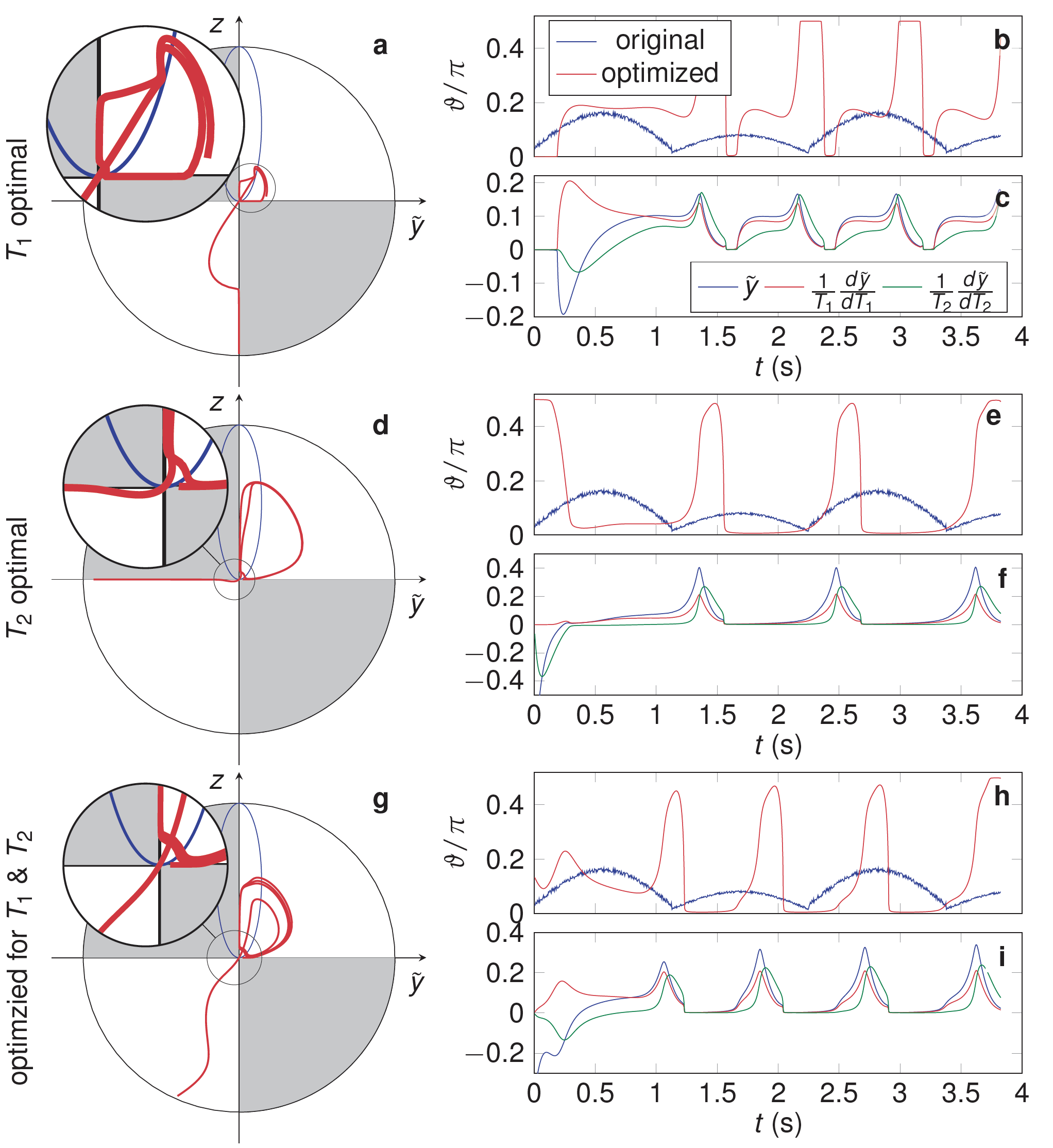
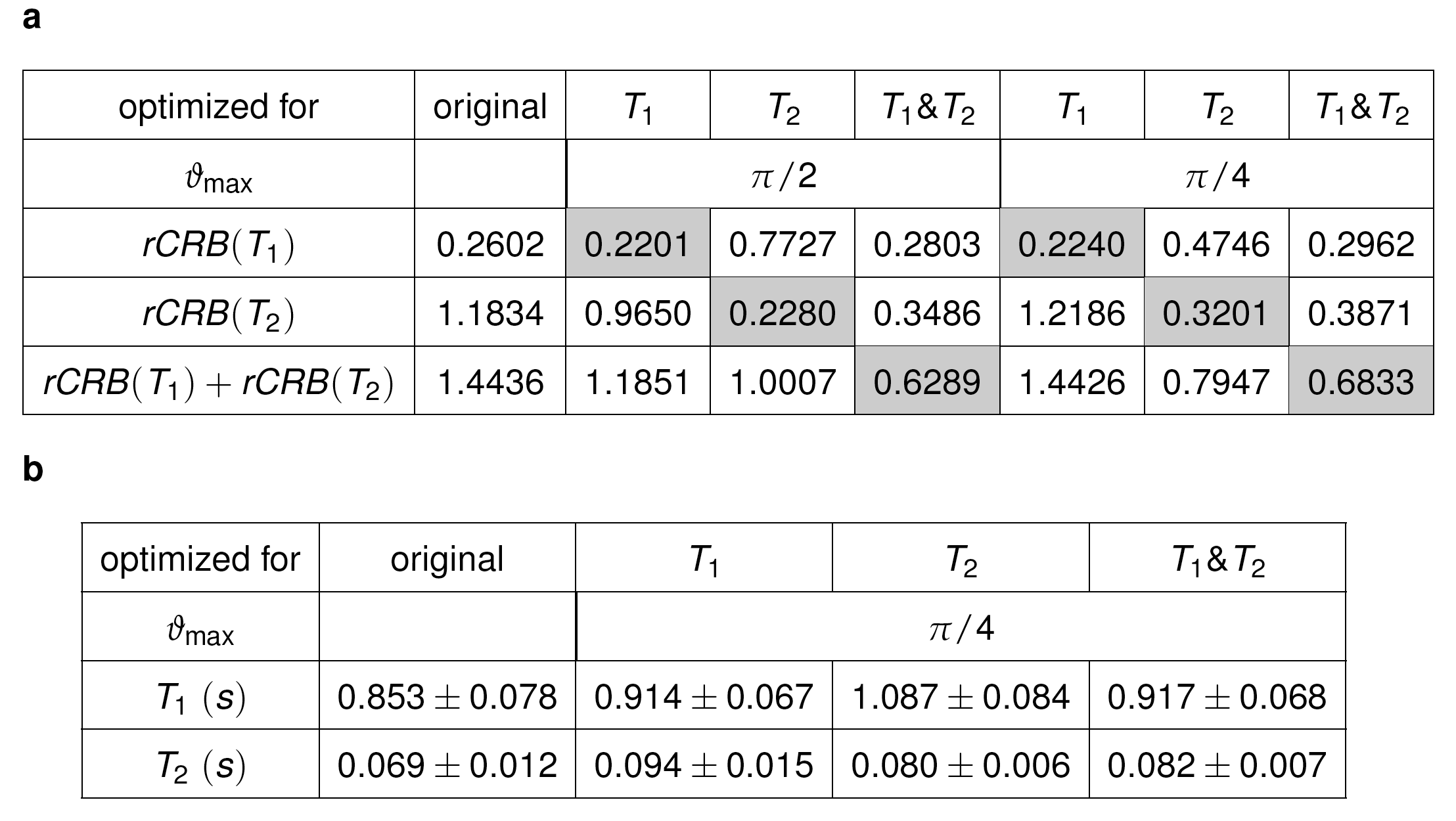
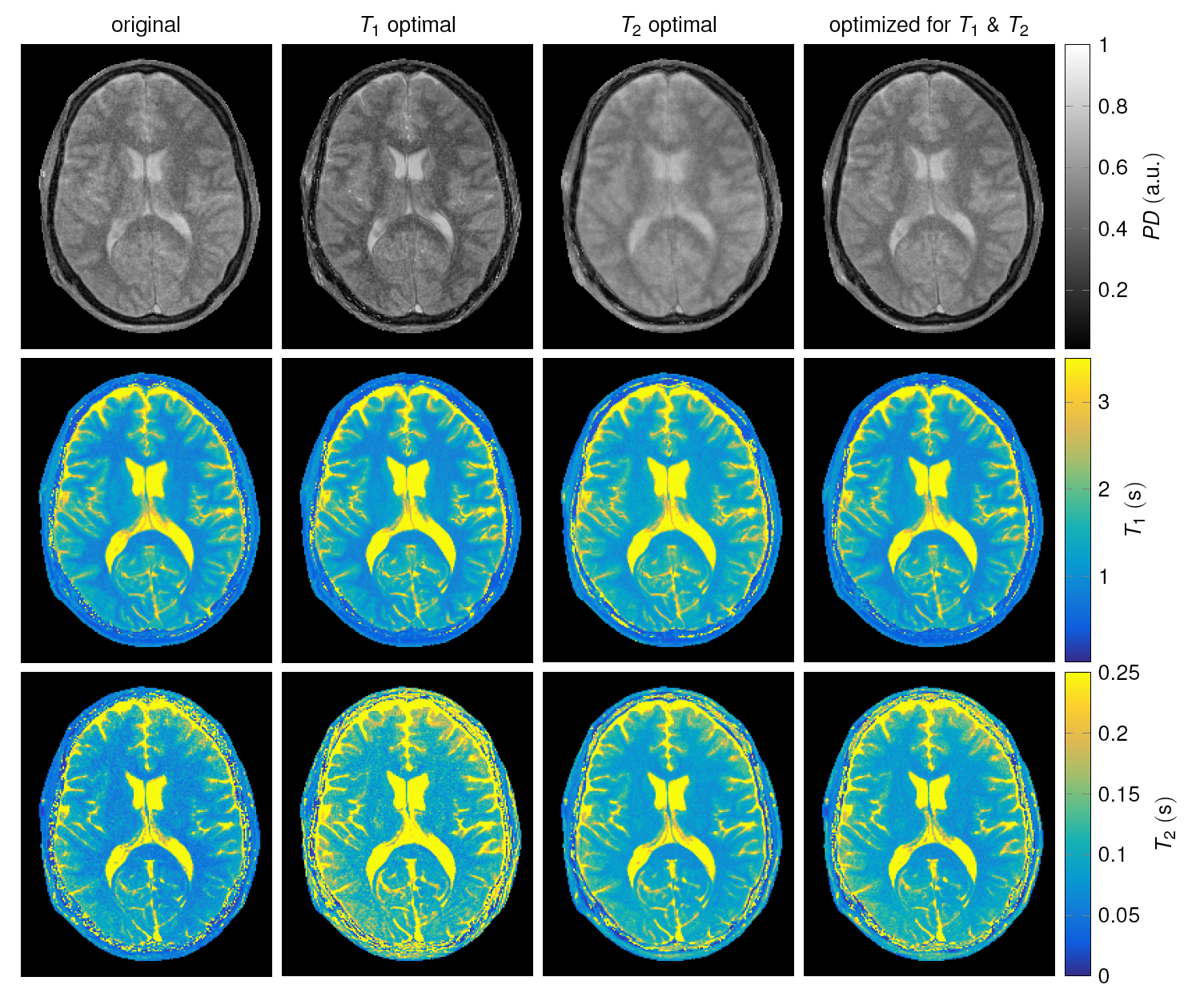
Numerical optimizations were performed with the optimal control10,11 based on the Bloch equations in polar coordinates. The Cramer-Rao bound was used as an objective function, which is based on the Fischer-information matrix $$$\mathbf{F}\in\mathbb{R}^{3\times3}~$$$with the entries$$$~\mathbf{F}_{i,j}=\mathbf{b}_i^T\mathbf{b}_j/\sigma^2~$$$,where $$$\mathbf{b}_1=\tilde{\mathbf{y}}=\mathbf{r}\sin{\boldsymbol{\vartheta}},\;\mathbf{b}_2=d\tilde{\mathbf{y}}/dT_1,\;\mathbf{b}_3=d\tilde{\mathbf{y}}/dT_2~$$$and$$$~\mathbf{r},\boldsymbol{\vartheta}\in\mathbb{R}^T~$$$are vectors describing the magnetization at $$$T$$$ measured time points. By normalizing with the input variance $$$\sigma^2$$$ and the relaxation time, we can define the relative Cram\'er-Rao bounds$$rCRB(T_1)=\frac{(\mathbf{F}^{-1})_{2,2}}{\sigma^2T_1^2}$$$$rCRB(T_2)=\frac{(\mathbf{F}^{-1})_{3,3}}{\sigma^2T_2^2}.$$These objective functions provide a measure for the noise transfer ($$$\sigma_{T_{1,2}}^2\geq{rCRB(T_{1,2})}\cdot\sigma^2\cdot{T_{1,2}^2}$$$) and are minimized with the Broyden-Fletcher–Goldfarb-Shanno algorithm.Optimizations were performed for $$$rCRB(T_1),rCRB(T_2)$$$ and $$$rCRB(T_1)+rCRB(T_2)~$$$with the relaxation times of white matter $$$T_1={0.781}\text{s},T_2={0.065}\text{s}$$$2. An inversion pulse at the beginning of the sequence defines $$$r(0)=-1$$$. All optimizations were initialized with the pattern provided in the pseudo-SSFP paper7 and were performed with $$$0\leq\vartheta\leq\pi/2$$$ and $$$0\leq\vartheta\leq\pi/4$$$, where the latter limits the flip angle to $$$\alpha\leq\pi/2$$$, ensuring compliance with safety considerations and consistent slice profiles.A healthy volunteer's brain was imaged with IRB-approval. Measurements were performed with the original pseudo-SSFP pattern and the pattern that minimize $$$rCRB(T_1),rCRB(T_2)$$$ and $$$rCRB(T_1)+rCRB(T_2)$$$, limited to $$$0\leq\vartheta\leq\pi/4$$$ (Figure$$$~$$$3). The flip angles are given by $$$\alpha(t_i)=\vartheta(t_i)+\vartheta(t_{i-1})$$$ and TR and TE were calculated according to the pseudo-SSFP7 framework with $$$TR_0=4.5\text{ms}$$$. The resolution of the maps is $$$1\text{mm}\times1\text{mm}\times3\text{mm}$$$. In total, 840 radial spokes were acquired with golden angle increment12 and image reconstruction was performed according to13. The total acquisition time was approximately $$$3.8\text{s}$$$.Results and Discussion
Initialized with strongly fluctuating excitation pattern, the optimized curves are comparably smooth (Figure$$$~$$$2b,e,h). The spin dynamics directly after the inversion pulse depends on the optimized objective as depicted on the Bloch-sphere. Optimizing for$$$~T_1$$$, the magnetization first relaxes along the$$$~z$$$-axis, providing no signal, before it follows a pear shape (Figure$$$~$$$3a). Optimizing for$$$~T_2$$$, the magnetization relaxes along the$$$~\tilde{y}$$$-axis (d), while in the combined optimization, it has a snack-like trajectory (g). For$$$~r,z>0$$$, the magnetization follows a circular trajectory that repeats itself. Its size and shape depends on the optimized parameter. The subplots (c,f,i) compares the encoding of the elements of the Fisher information matrix. When limiting$$$~\vartheta$$$, the general nature of the trajectories remains unchanged (Figure$$$~$$$3). The original pseudo-SSFP pattern has a good performance in encoding $$$~T_1~$$$,while$$$~T_2~$$$is comparably noisy7. This is confirmed by the$$$~rCRB~$$$(Table$$$~$$$1a). Optimizing for $$$T_2$$$ decreases the sensitivity to$$$~T_1~$$$,while a combined optimization greatly improves$$$~T_2~$$$with minor sacrifices in$$$~T_1~$$$. This is confirmed by the visual impression of the in vivo data (Figure$$$~$$$4) and by the standard deviation within a region of interest (Table$$$~$$$1b). Systematic errors can be noted in the measured relaxation times, which are most likely caused by slice-profile imperfections and magnetization transfer, which are not addressed in the present work.Conclusion
Describing the spin dynamics in polar coordinates provides insights in the spin dynamics in balanced non-steady-state sequences. The excitation angle can be seen as a control parameter, which provides indirect access to the relaxation in the radial direction. Further, it is shown that TR has no effect on the relaxation within certain limits and that numerical optimizations based on polar coordinates show robust convergence. Future work will include an in-depth analysis of the shape of the spin-trajectory on the Bloch-sphere as a function of various parameters.Acknowledgements
The Authors would like to thank Steffen Glaser, Quentin Ansel and Dominique Sugny for the fruitful discussions about optimal control and for giving insights in their implementations.
This work was supported in part by the research grants NIH R21 EB020096 and was performed under the rubric of the Center for Advanced Imaging Innovation and Research(CAI2R, www.cai2r.net), a NIBIB Biomedical Technology Resource Center(NIH P41 EB017183).
References
[1] Dan Ma, Vikas Gulani, Nicole Seiberlich, Kecheng Liu, Jeffrey L. Sunshine, Jeffrey L. Duerk, and Mark A. Griswold. Magnetic resonance fingerprinting. Nature,495(7440):187–192, 2013.
[2] Yun Jiang, Dan Ma, Nicole Seiberlich, Vikas Gulani, and Mark A. Griswold. MR fingerprinting using fast imaging with steady state precession (FISP) with spiral readout. Magnetic Resonance in Medicine, 74:1621–1631, 2015.
[3] M Cloos, F Knoll, T Zhao, K. Block, M. Bruno, CG Wiggins, and Daniel K. Sodickson. Multiparamatric imaging with heterogenous radiofrequency fields. Nature Commnuication, in press:DOI: 10.1038/ncomms12445, 2016.
[4] Ouri Cohen, Mathieu Sarracanie, Brandon D. Armstrong, Jerome L. Ackerman, and Matthew S. Rosen. Magnetic Resonance Fingerprinting Trajectory Optimization. In Proc. Intl. Soc. Mag. Reson. Med. 22, page 0027, 2014.
[5] Bo Zhao, Justin P Haldar, Kawin Setsompop, and Lawrence L Wald. Optimal Experiment Design for Magnetic Resonance Fingerprinting. (1):453–456, 2016.
[6] Ouri Cohen, Mathieu Sarracanie, Matthew S. Rosen, and Jerome L. Ackerman. In Vivo Optimized Fast MR Fingerprinting in the Human Brain. In Proc. Intl. Soc. Mag. Reson. Med. 24, page 430, 2016.
[7] Jakob Assländer, Steffen J Glaser, and Ju¨rgen Hennig. Pseudo Steady-State Free Precession for MR-Fingerprinting. Magnetic Resonance in Medicine, page epubahead of print, 2016.
[8] Klaus Scheffler and Jürgen Hennig. Is TrueFISP a gradient-echo or a spin-echo sequence? Magnetic Resonance in Medicine, 49(2):395–397, feb 2003.
[9] Jürgen Hennig, Oliver Speck, and Klaus Scheffler. Optimization of signal behavior in the transition to driven equilibrium in steady-state free precession sequences. Magnetic Resonance in Medicine, 48(5):801–809, 2002.
[10] S Conolly, D Nishimura, and A Macovski. Optimal control solutions to the magnetic resonance selective excitation problem. IEEE Transactions on Medical Imaging, 5(2):106–115, 1986.
[11] Thomas E Skinner, Timo O Reiss, Burkhard Luy, Navin Khaneja, and Steffen J Glaser. Application of optimal control theory to the design of broadband excitation pulses for high-resolution NMR. Journal of Magnetic Resonance, 163(1):8–15, 2003.
[12] Stefanie Winkelmann, Tobias Schaeffter, Thomas Koehler, Holger Eggers, and Olaf Doessel. An Optimal Radial Profile Order Based on the Golden Ratio for Time-Resolved MRI. IEEE Transactions on Medical Imaging, 26(1):68–76, jan 2007.
[13] Jakob Assländer, Martijn A Cloos, Florian Knoll, Daniel K Sodickson, Jürgen Hennig, and Riccardo Lattanzi. Low Rank Alternating Direction Method of Multipliers Reconstruction for MR Fingerprinting. preprint, page arXiv:1608.06974, 2016.
Figures