Introduction

In the field of musculoskeletal MRI, phase-contrast sequences have been applied to quantify inter alia change in fascicle length¹, strain rates², and inertial forces³. More specifically, time-resolved 3D phase-contrast imaging can be used to quantify muscle contraction in an entire 3D volume of muscle groups. 3D coverage with sufficient spatiotemporal resolution (~3x3x5 mm³, 160 ms) can only be achieved by interleaved acquisitions during many repetitions of a motion task, resulting in long scan times (>10 min). The many repetitions of the motion task may result in muscle fatigue resulting in poor reproducibility and hampering applications in diseased or injured subjects. The application would greatly benefit from acceleration to reduce the total acquisition time. The aim of this study was therefore to develop a Compressed Sensing (CS)^4,5 accelerated time-resolved 3D phase-contrast MRI technique for quantifying velocities of the muscles in the lower leg during active foot plantar- and dorsiflexion.

Methods

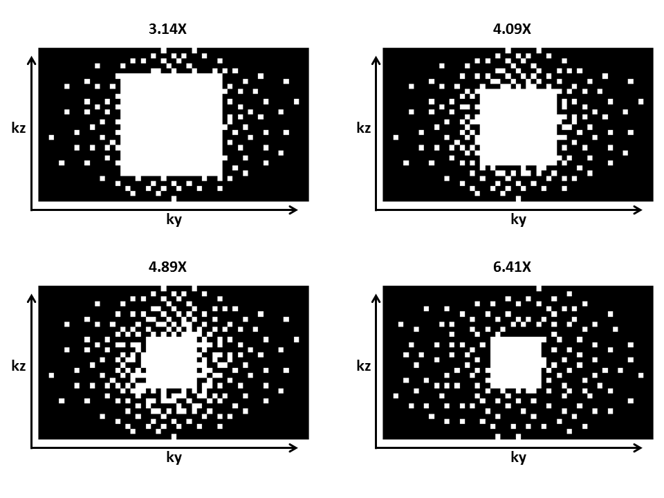
Four healthy volunteers with no history of muscle pain and abnormalities in the lower leg were scanned with an Ingenia 3T MRI scanner (Philips Healthcare, Best, Netherlands) using a 16-channel Torso and 12-channel posterior coil. Subjects were placed supine, feet first in the scanner. After high-resolution anatomical mDIXON scan at rest, the volunteers were instructed to make continuous smooth movements with the right foot between 20° dorsiflexion to 20° plantarflexion. Five time-resolved 3D turbo field echo (TFE) phase-contrast acquisitions were executed; one fully sampled and four accelerated acquisitions. The volunteers received a visual cue from a bouncing ball displayed on a screen with a cycle duration of 2000 ms to guide their motion task. The MRI scan was triggered at the same pace. Scan parameters for the fully sampled 3D TFE scan were TFE-factor of 3, half scan in phase-encoding direction of 0.6, matrix size of 153x53x30, voxel size of 3x3x5 mm³, TE/TR of 4.5/6.4 ms, VENC of 12 cm/s in three orthogonal directions (FH, AP, LR), and a temporal resolution of 160 ms. Accelerated acquisitions were performed with the same parameters, except for the half scan, but different k-space undersampling schemes (acceleration factors: 3.14, 4.09, 4.89, and 6.41X) as shown in Figure 1. The scanner software was modified to acquire a predefined number of sampling profiles. The sampling profiles (ky,kz) were generated in MATLAB (The MathWorks Inc., Natick, MA, USA) using the Berkeley Advanced Reconstruction Toolbox (BART)⁶ and were designed according to a Poisson-disc pattern with variable density. Total acquisition times for the five scans were 10:52 (fully), 5:38, 4:20, 3:38, and 2:46 min. Raw data was imported to MATLAB using ReconFrame (Gyrotools, Zurich, CH) and CS reconstruction was performed using the BART with a wavelet transform in space (x,y,z) and an additional sparsifying total variation (TV) transform in space (x,y,z) and time. The L1-regularization was performed with a regularization parameter of r=0.01 and 50 iteration steps.

Results

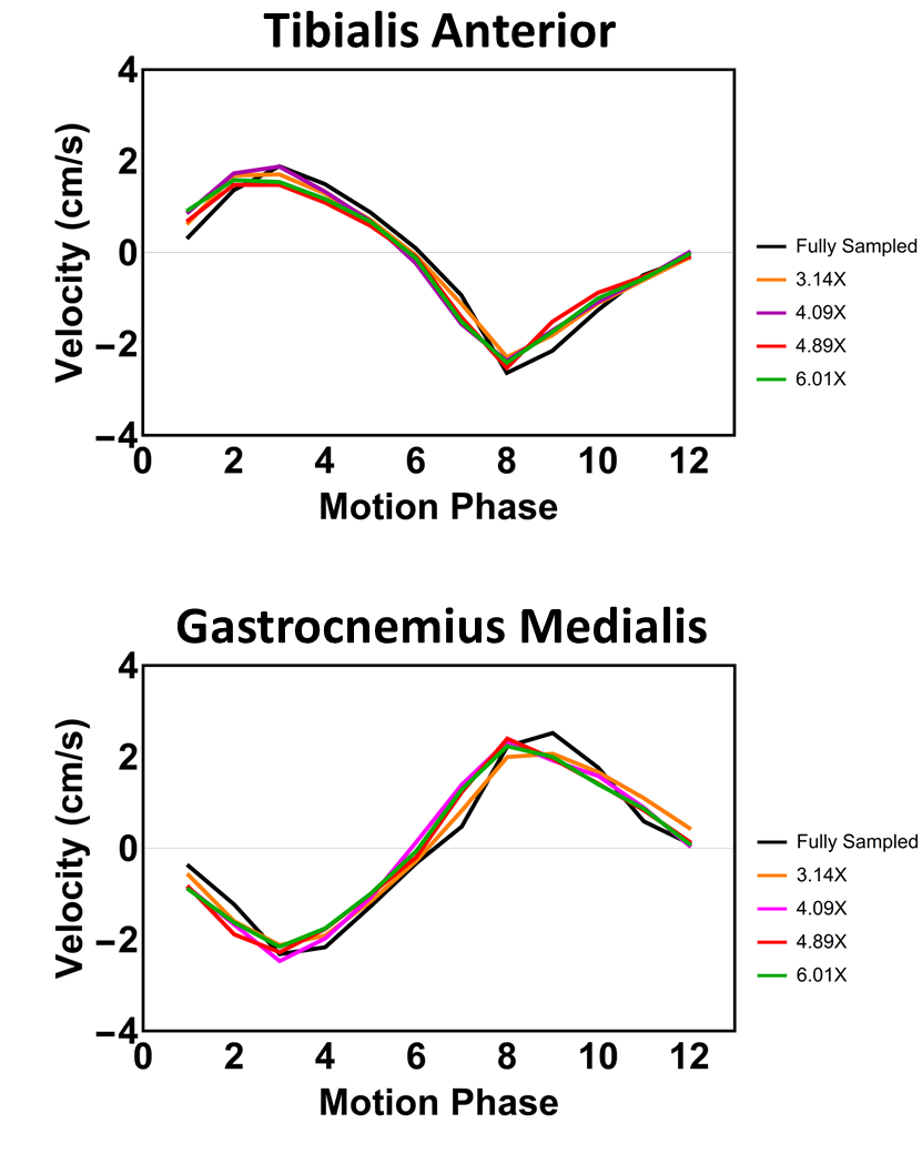
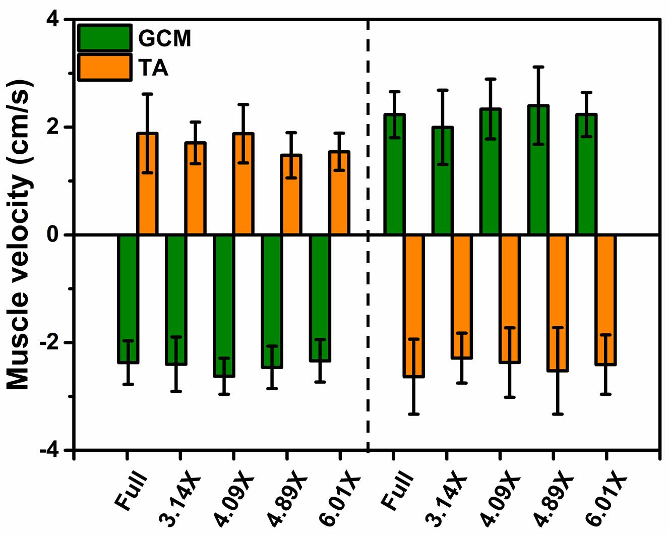
Figure 2 shows magnitude and velocity images reconstructed from undersampled data in comparison to a fully sampled data set. Velocity difference maps between accelerated and fully sampled data are shown for one volunteer for all frames. Temporal mean velocity differences over a region-of-interest in the Tibialis Anterior (TA) muscle range for all volunteers maximal between 2.7% (3.14X) and 3.9% (6.41X). Figure 3 depicts velocity curves averages over all volunteers of the dorsi- and plantarflexion cycle for both the full TA and the Gastrocnemius Medialis (GCM) muscle. No apparent deviations from the fully sampled scan are recognizable up to an acceleration factor of 6.41X. For all volunteers, the mean and standard deviation of the velocity curves were calculated in Figure 4 for both TA and GCM muscles for two frames belonging to the climax of dorsi- or plantarflexion, respectively. No significant differences are observed for different acceleration factors. Figure 5 shows a 3D visualization of the measured velocities in four transverse slices, illustrating the motion of the TA and GCM muscle in opposite direction.

Discussion

Difference images comparing undersampled time resolved 3D PC-MRI data to fully sampled data shows no substantial difference, even up to an acceleration factor of 6.41X. Although deviations in the velocity curves for in single frames may exist, on average fully sampled and highly undersampled data provide the same results, thus facilitating a significant decrease in scan time from 10:52min down to 2:46min (6.41X).

Conclusion

This study demonstrated that it is possible to reconstruct highly undersampled Cartesian PC data of the muscles in the lower leg during active plantar- and dorsiflexion using compressed sensing. This strategy facilitates a significant decrease in scan time while keeping comparable image quality.

Acknowledgements

N/A