0085
Absolute MR Thermometry from Multi-Echo GRE with B0-Correction1Electrical Engineering and Computer Science, Massachusetts Institute of Technology, Cambridge, MA, United States, 2Athinoula A Martinos Center for Biomedical Imaging, Massachusetts General Hospital, Charlestown, MA, United States, 3Radiology, Harvard Medical School, Boston, MA, United States, 4Radiology, Boston Children’s Hospital, Boston, MA, United States, 5Pediatrics, Boston Children's Hospital, Boston, MA, United States, 6Institute for Medical Engineering and Science, Massachusetts Institute of Technology, Cambridge, MA, United States
Synopsis
MR thermometry offers the potential to obtain absolute and relative temperature measurements on a voxelwise basis, but is affected by B0 offsets. Since precise (<1°C) temperature measurements are important for simulation validation in phantom experiments, and since realistic phantoms and models have regions of high ΔB0 , there is a need for accurate, B0-robust temperature mapping methods. In this work, we propose such a method using a multi-TE GRE acquisition and validate it in phantom experiments.
Introduction
MR thermometry can be used to verify thermal simulations, as has been done in prior studies on MR safety. Since regulatory bodies impose limits on temperature increase during MRI of 0.5°C to 2.0°C , and since real anatomy and realistic phantoms contain regions of high B0 offset, there is a need for accurate, B0-robust temperature mapping. Previous work in this field has explored using multi-echo GRE for temperature mapping [1], but this approach is susceptible to B0-induced errors in temperature measurements. Here, we propose a method for B0-robust absolute temperature mapping and validate it by experiments on an Ethylene Glycol phantom.
Theory
For certain two-species spin systems (including Ethylene Glycol [2]), temperature is linearly related, by a known constant, to the difference in resonance frequency between the two resonances, $$$\Delta{f}$$$ . A method for measuring $$$\Delta{f}$$$ for two-species systems from multi-echo GRE data [1] has previously been demonstrated. However, due to the inter-species resonance difference and finite readout bandwidth, a reconstructed voxel signal in a GRE acquisition is the sum of two signals from two chemical species at different spatial locations. If these two locations have different main field offsets $$$\Delta {B}_{0}$$$ , then the difference in the locations of the voxel signal’s spectral peaks will incorporate this spatial difference in $$$\Delta{B}_{0}$$$: $$\Delta{f}_{Meas}(x) = \Delta{f}_{True}(x)+ \frac{\gamma}{2\pi}(\Delta{B}_{0}(x)-\Delta{B}_{0}(x+\delta{x}(x))) $$ The spatial shift at a given location ($$$\delta{x}(x)$$$), in pixels, is: $$\delta{x}(x)=\frac{\Delta{f}_{True}(x)}{BW}$$ Where $$$BW$$$ is the readout pixel bandwidth. In a typical thermometry experiment, we expect the phantom temperature to vary no more than a few degrees (<5°C) from the starting temperature. Thus, we simplify this equation by assuming that: $$$\Delta{f}_{True}(x)=\Delta{f}(T={T}_{room})$$$ for all $$$x$$$. Using multi-echo GRE data, it is possible to measure both $$$\Delta{f}_{Meas}$$$ [1] and $$$\Delta{B}_{0}$$$. From $$$\Delta{B}_{0}$$$ we calculate the error term and subtract it to obtain $$$\Delta{f}_{True}(x)$$$ . Using this, we obtain a $$${B}_{0}$$$-corrected temperature map.
Methods
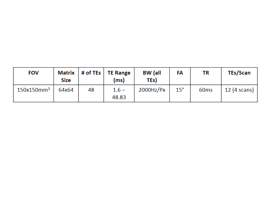
Experiments were performed on spherical (7.6cm and 5cm outer diameter) ethylene glycol phantoms. Data were acquired in two different experiments with the protocol in Table 1. The phantoms were placed so as to induce $$${B}_{0}$$$ variations in each other. All data were acquired on a Siemens 3T Trio system using the product 32-channel head receive array and used monopolar readout gradients.
1. The phantoms were kept in the scanner room for over 24 hours prior to scanning and were assumed to be at a constant temperature during the scan. Phantom temperature was measured with a temperature probe before and after the scan. Data were acquired five times in succession.
2. The phantoms were placed near a bath of ice water to induce cooling in the phantom. Data were acquired at 15 sample times separated by approximately 2 minutes. Field maps were recalculated for each time point and were used in further analyses. A two-peak fit was applied following [1]. Field maps were calculated using the same GRE data, and temperature maps were corrected as described. Analysis was performed in MATLAB.
Results
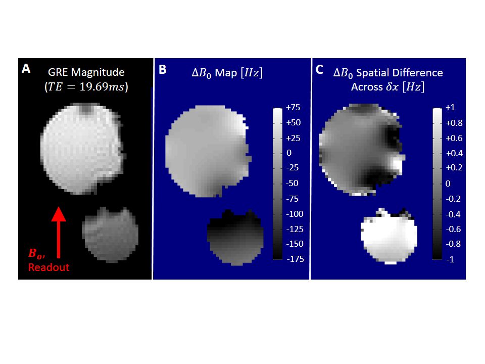
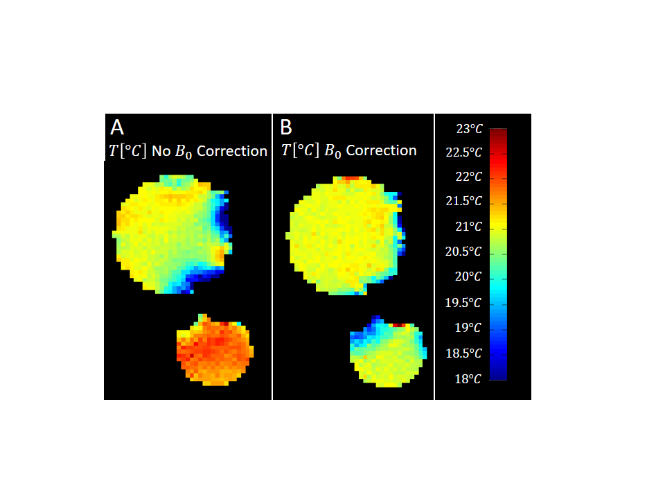
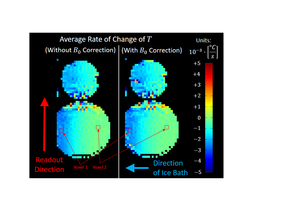
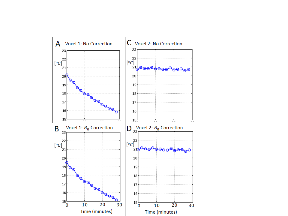
The phantoms were measured to be 21±0.5°C prior to the scan. GRE magnitude and $$$\Delta{B}_{0}$$$ are shown in Figures 1A and 1B. The spatial difference in $$$\Delta{B}_{0}$$$ (Figure 1C) visible matches the temperature map reconstructed without $$${B}_{0}$$$ -correction (Figure 2A). The temperature map reconstructed with $$${B}_{0}$$$-correction (Figure 2B) is more uniform than that without it. The average and standard deviation temperatures were 20.9°C and 0.69°C, respectively, without $$${B}_{0}$$$-correction. They were 20.8°C and 0.33°C, respectively, with it. The mean temperatures in the smaller and larger spheres were 21.8°C and 20.7°C without $$${B}_{0}$$$-correction, and 20.6°C and 21.0°C with it. Voxelwise standard deviation across time was, on average across the whole FOV, 0.09°C both with and without $$${B}_{0}$$$-correction. In the cooling experiment, the side of the phantom near the ice bath underwent cooling, while the side opposite the ice bath had minimal change in temperature (Figure 3). Temperature time series are shown for a voxel that did undergo cooling (Figures 4A and 4B) and one that did not (Figures 4C and 4D). The measured changes across the experiment for the “cooling” voxel were: -4.32°C (without $$${B}_{0}$$$-correction) and -4.32°C (with $$${B}_{0}$$$-correction).Conclusion
We also demonstrate a temporal precision of 0.1°C for relative temperature measurements with and without $$${B}_{0}$$$-correction. Spatial variation in temperature measurements from a uniform temperature phantom was reduced by 50% using $$${B}_{0}$$$-correction. The bias in temperature estimates was less than 0.5°C (the absolute validation precision) with $$${B}_{0}$$$-correction, but was 1.0°C off in the small phantom without it. These measurements are for a 16-second, single-slice 64x64 acquisition at 2.3x2.3mm2 voxel size.Acknowledgements
NIH R01EB017337, NIH U01HD087211References
[1] Sprinkhuizen SM, Bakker CJG, Bartels LW. Absolute MR Thermometry Using Time-Domain Analysis of Multi-Gradient-Echo Magnitude Images. MRM 2010. [2] Amman C, Meier P, Merbach AE. A simple multinuclear NMR thermometer. J Magn Reson 1982.Figures