0079
Thermal Variation and Temperature-Based Prediction of Gradient Response1Institute for Biomedical Engineering, University of Zurich and ETH Zurich, Zurich, Switzerland
Synopsis
Under the assumption that a gradient system is linear and time-invariant (LTI), accurate gradient field waveforms can be predicted by gradient response functions. However, time-invariance can be violated due to heating of system components. Temperature sensors can be used to assess heating of the gradient coils. To assess the predictability of gradient response function based on temperature measurements, the temperature dependence of gradient response functions is analyzed using an NMR probe based field camera and optically connected temperature sensors. From this data a prediction model is generated and tested for its application in image reconstruction.
Introduction
The vast majority of advanced MR imaging methods depends on very accurate gradient waveforms for signal encoding and preparation. Many hardware factors limit the fidelity of these waveforms, such as eddy currents, limited bandwidth and mechanical vibrations. Under the assumption that these systems are linear time-invariant (LTI), the actual gradient field waveforms of an ideal input pulse program can be calculated using gradient response functions [1–3] and be used for image reconstruction [3]. Recent research showed that the assumption of time-invariance can be violated under high duty-cycles presumably due to heat up of the MR system components [4, 5]. These changes, however, are slow compared to typical imaging readouts and may be mapped to temperature distributions as suggested by [4]. To assess the predictability of gradient response function based on temperature measurements we analyze temperature related changes on an extended dataset and use the resulting model to perform gradient response predictions over periods of weeks, solely based on response function calibration data and temperature sensor data.Methods
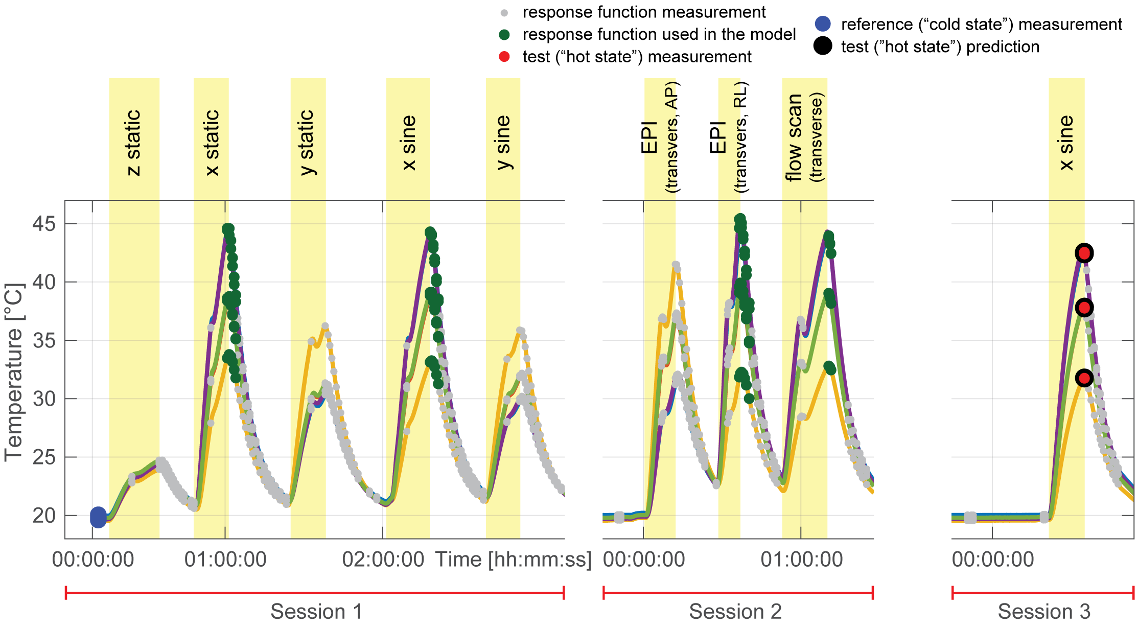
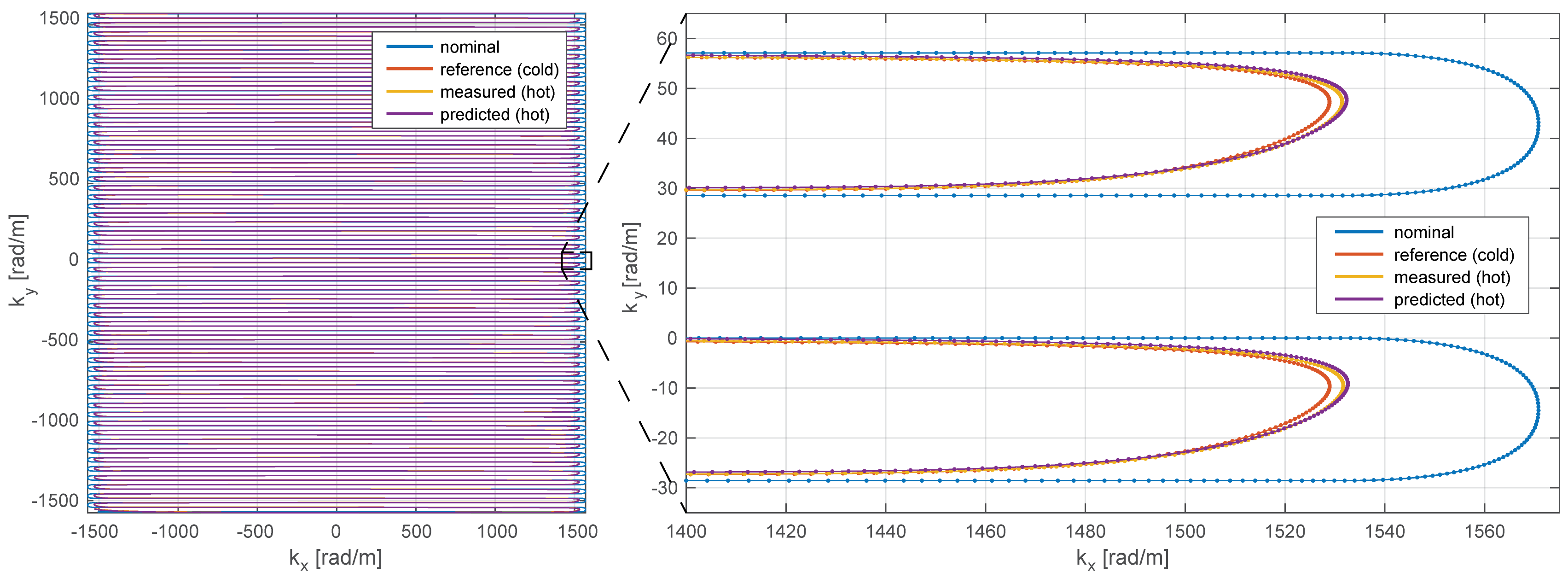
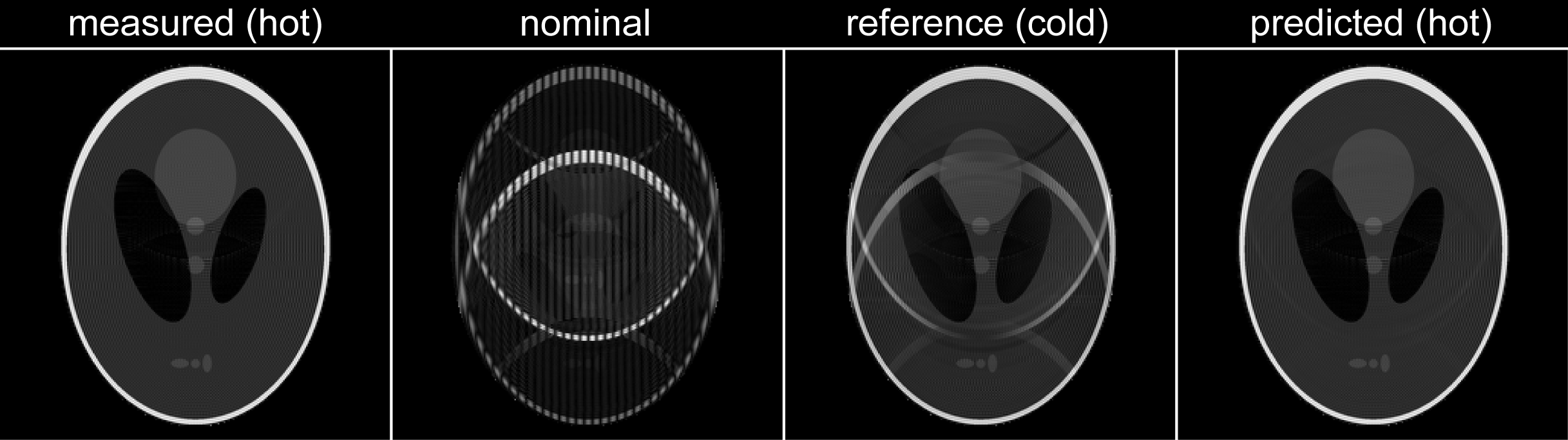
In order to measure response functions, frequency swept pulses (0-30kHz, duration: 100ms) were played out on each gradient input [2] and the corresponding field responses were measured over a period of 1.1s. A recently proposed continuous field monitoring method [6], based on rapidly re-excited sets of NMR probes [7, 8] and a dedicated monitoring system [9] was used to capture the field responses. This method enables fast, high SNR, single-shot field measurements over arbitrary durations. The actual response functions were then determined by deconvolution in the frequency domain. Measurements from 5 optically connected temperature sensors (casted into the gradient coil) were used to monitor the temperature with a temporal resolution of 1 s. In two calibration sessions response functions were measured under various temperature distributions, which were reached by playing out different heating gradient waveforms as illustrated in Figure 1. This calibration data set was then used to predict response functions in a third session from the current temperature (Figure 1). The employed prediction model was based on the temperatures ($$$T$$$), the derivative of the temperatures ($$$\dot{T}$$$) and GIRFs ($$$G$$$) from similar temperature conditions: $$$G=B_0+B_1 T+B_2 \dot{T}$$$, with $$$B_0$$$ a constant component, $$$B_1$$$ the temperature dependent components and $$$B_2$$$ the temperature derivative dependent components, all represented in the frequency domain. The training GIRFs ($$$G$$$) with similar temperature conditions were selected based on their Euclidean distance to the test temperature condition in the 5 dimensional temperature space spanned by the 5 temperature sensors. The radius of this selection range was set to 8 °C. The quality of the predicted GIRFs was assessed by image reconstruction on simulated data. Therefore, four different k-space trajectories were employed. A nominal trajectory (resolution = 1mm, FOV = 256mm, duration = 59ms, SENSE 2.32) as well as “cold state”, “hot state” and “hot state temperature predicted” trajectories that were calculated from the corresponding response functions and the gradients of the nominal trajectory. Thereafter NMR signals of an object were first simulated based on the “hot state” trajectory $$$k(t)$$$ as $$$M(t) = s(x)A(x) e^{i k(t)x}$$$. With $$$k$$$ being the k-space coordinates, $$$s$$$ coils sensitivities and $$$A$$$ the objects transverse magnetization. Subsequently images were reconstructed on a 256x256 matrix with all four trajectories. Image reconstruction was based on the iterative SENSE reconstruction described in [10, 11]. All measurements were performed on a Philips Achieva 7T MRI system (Philips Healthcare, Cleveland, USA).Results
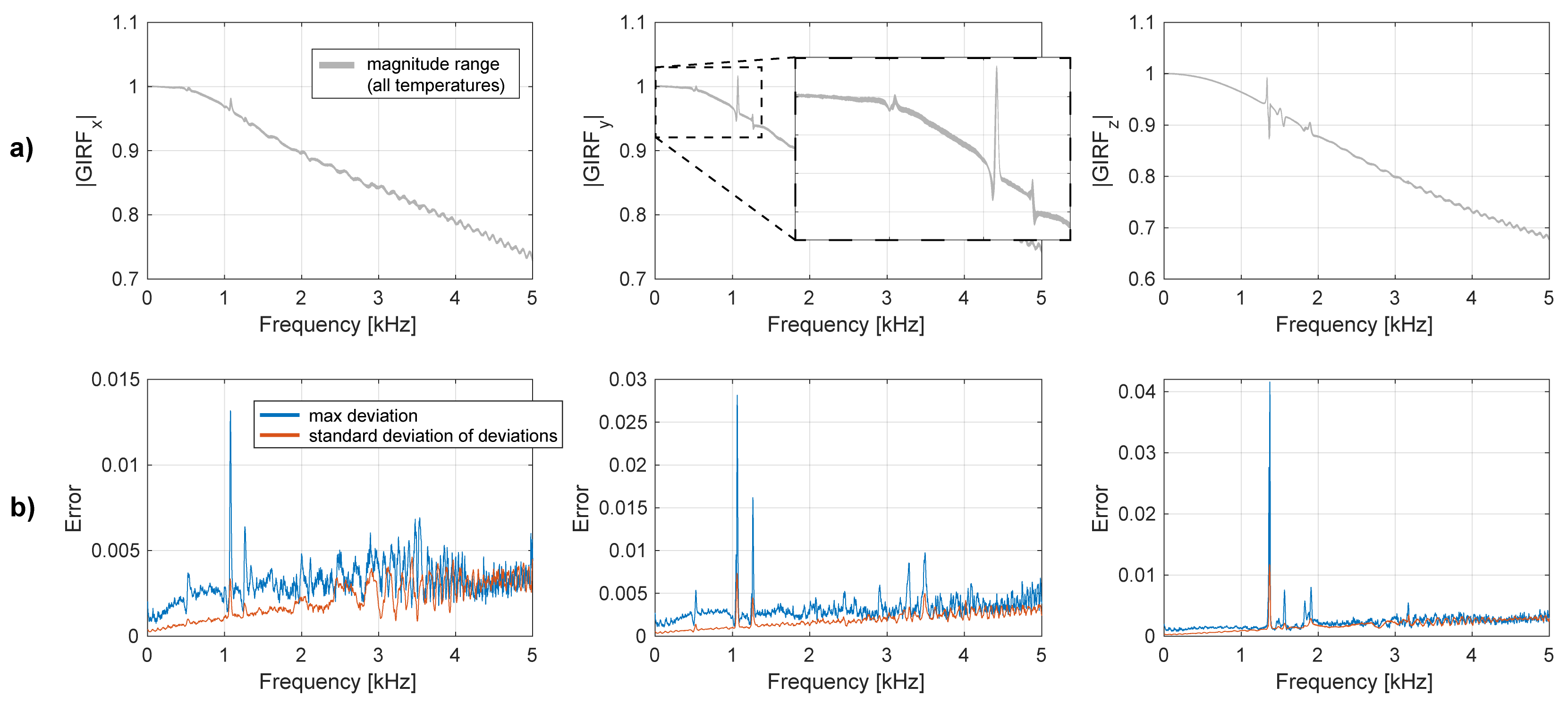
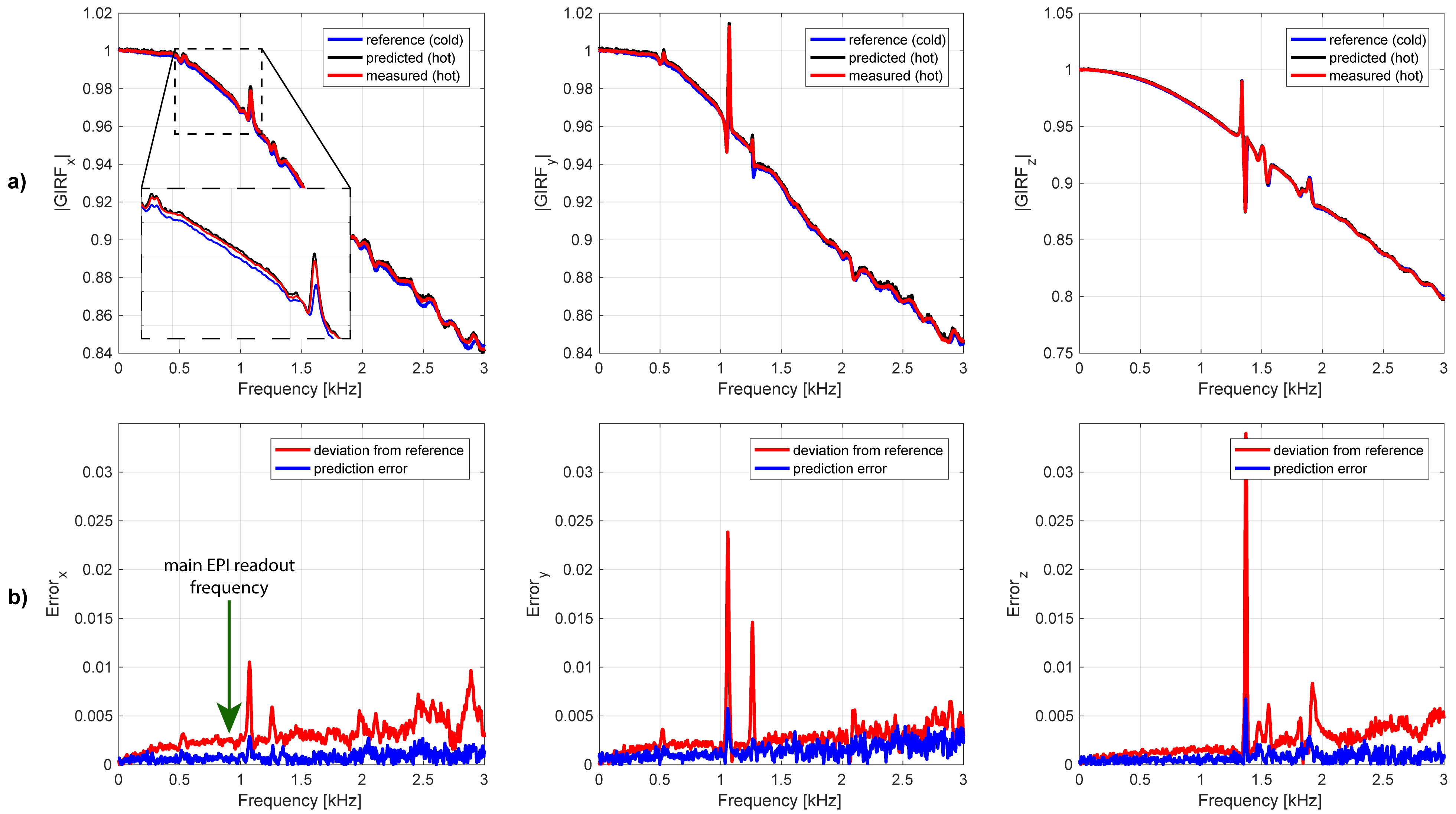
Figure 1 shows that heating curves look quite different depending on the input gradient waveforms. The smallest overall heat-up is observed on the z-channel, which is probably due to direct water cooling of the conductor. The deviations of the observed response functions under different temperatures span a range of up to 4% at resonance frequencies (most likely mechanical) and up to 5‰ in the most relevant band for imaging sequences of up to 5kHz (Figure 2). It can be seen in Figure 4 that all response function based trajectories deviate significantly from the nominal trajectory due to the bandwidth limitations imposed by the system. The temperature predicted one does not fully match the one calculated with the “hot state” response function, but it gets significantly closer than the “cold state” trajectory. A clear improvement of the temperature based prediction compared to the “cold state” and nominal can be observed in the corresponding images (Figure 5).Discussion / Conclusions
Time-invariance violations of gradient response functions due to temperature changes were analyzed and response functions of “hot” system states successfully predicted using a model based on previously acquired calibration data at similar temperature conditions.Acknowledgements
No acknowledgement found.References
[1] S. J. Vannesjo, M. Haeberlin, L. Kasper, M. Pavan, B. J. Wilm, C. Barmet, and K. P. Pruessmann, “Gradient system characterization by impulse response measurements with a dynamic field camera,” Magn. Reson. Med, vol. 69, no. 2, pp. 583–593, 2013.
[2] S. J. Vannesjo, B. E. Dietrich, M. Pavan, D. O. Brunner, B. J. Wilm, C. Barmet, and K. P. Pruessmann, “Field camera measurements of gradient and shim impulse responses using frequency sweeps,” Magn. Reson. Med, vol. 72, no. 2, pp. 570–583, 2014.
[3] S. J. Vannesjo, N. N. Graedel, L. Kasper, S. Gross, J. Busch, M. Haeberlin, C. Barmet, and K. P. Pruessmann, “Image reconstruction using a gradient impulse response model for trajectory prediction,” Magn Reson Med, 2015.
[4] B. E. Dietrich, J. Reber, D. O. Brunner, B. J. Wilm, and K. P. Pruessmann, “Analysis and Prediction of Gradient Response Functions Under Thermal Load,” in Proc Int Soc Magn Reson Med Sci Meet Exhib, 2016, p. 3551.
[5] J. Busch, S. J. Vannesjo, C. Barmet, K. P. Pruessmann, and S. Kozerke, “Analysis of temperature dependence of background phase errors in phase-contrast cardiovascular magnetic resonance,” J Cardiovasc Magn Reson, vol. 16, p. 97, 2014.
[6] B. Dietrich, D. Brunner, B. Wilm, C. Barmet, and K. Pruessmann, “Continuous magnetic field monitoring using rapid re-excitation of NMR probe sets,” IEEE Trans Med Imaging, vol. 35, no. 6, pp. 1452–1462, 2016.
[7] C. Barmet, N. De Zanche, and K. P. Pruessmann, “Spatiotemporal magnetic field monitoring for MR,” Magn. Reson. Med, vol. 60, no. 1, pp. 187–197, 2008.
[8] N. De Zanche, C. Barmet, J. A. Nordmeyer-Massner, and K. P. Pruessmann, “NMR probes for measuring magnetic fields and field dynamics in MR systems,” Magn. Reson. Med, vol. 60, no. 1, pp. 176–186, 2008.
[9] B. E. Dietrich, D. O. Brunner, B. J. Wilm, C. Barmet, S. Gross, L. Kasper, M. Haeberlin, T. Schmid, S. J. Vannesjo, and K. P. Pruessmann, “A field camera for MR sequence monitoring and system analysis,” Magn. Reson. Med, vol. 75, no. 4, pp. 1831–1840, DOI: 10.1002/mrm.25770, 2016.
[10] K. P. Pruessmann, M. Weiger, M. B. Scheidegger, and P. Boesiger, “SENSE: sensitivity encoding for fast MRI,” Magn. Reson. Med, vol. 42, no. 5, pp. 952–962, 1999.
[11] K. P. Pruessmann, M. Weiger, P. Börnert, and P. Boesiger, “Advances in sensitivity encoding with arbitrary k-space trajectories,” Magn. Reson. Med, vol. 46, no. 4, pp. 638–651, 2001.
Figures