Synopsis

We introduce a general description of the RF response of an implant, defined as the implant response matrix (IRM). An analytical expression for the IRM is derived through basis functions that depend on a limited number of parameters. This analytical model is validated with a simulation study (Pearson correlation coefficients with simulations R: 0.9979-0.9996). This description allows a significant reduction in unknowns enabling IRM assessment by MRI measurements without hardware modifications to scanner or implant. The feasibility of MRI based IRM/TF measurement is shown in silico. With the simulated complex B₁⁺ fields the IRM is accurately reconstructed (R: 0.974).

Purpose

Theory

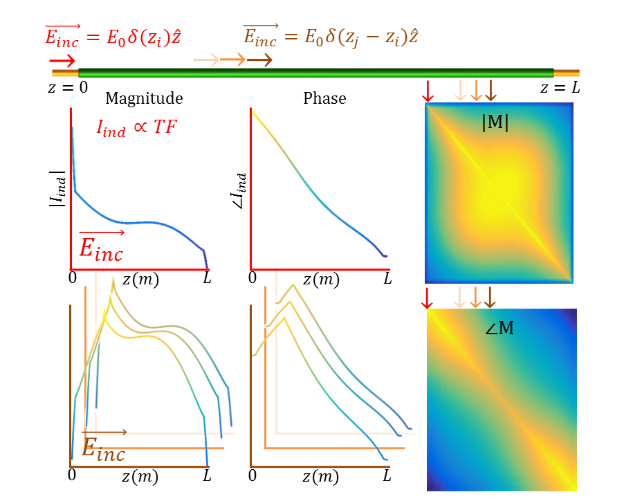
We define the implant response matrix $$$M\,$$$as$$$\,I_{ind}=ME_{inc}\,$$$where$$$\,I_{ind}\,$$$is a vector containing the induced current distribution along the implant and $$$E_{inc}$$$ is a vector with the incident, tangential electric field. This field induces an RF current in the implant as shown in figure 1. If this exposure is a point-excitation at the tip of the implant, the resultant current distribution in the implant directly reflects the TF of the implant³. If this excitation occurs at a different location,$$$z_j$$$, it will induce another current pattern. This scattering can be described by the IRM, $$$M$$$.

By definition, the induced current patterns in figure 1 are its columns. The parameter space of this matrix is greatly reduced when the current patterns are modeled by damped waves originating at the location of excitation. They repeatedly reflect at both ends of the implant. The summation of these waves leads to a converging geometric series. The IRM then becomes:$$\tag{1}M_{ij}=\sigma_{eff}E_{0}e^{-c|z_i-z_j|}+\frac{\sigma_{eff}E_{0}}{1-r_{0}r_{L}e^{-2cL}}[\sqrt{r_{0}r_{L}}e^{-cL}\cosh(c(z_i+z_j-L)-\frac{1}{2}\ln(\frac{r_{0}}{r_{l}}))+r_{0}r_{L}e^{-2cL}\cosh(c(z_i-z_j))],$$ $$$c$$$ is the complex propagation constant of the current wave in the implant of length $$$L$$$. $$$r_0$$$, and $$$r_L$$$, are the reflection coefficients. Hereby the IRM of an implant is described by four complex parameters. With additional parameters,$$$\{c_2,c_3,...,t_{12},t_{23},..\}$$$, similar equations can be derived for implants that consist of multiple segments resulting in additional transmissions and reflections.

Methods

Electromagnetic simulations (Sim4Life,ZMT, Zurich) were used to validate the theoretical model to describe the IRM. $$$M$$$ is determined by applying narrow (5mm) plane wave excitations with positively interfering electric fields at various positions $$$z_j$$$ along the implant and monitoring the induced current distribution in the elongated implant. The resultant $$$M$$$ is considered the ground truth representation of the IRM.

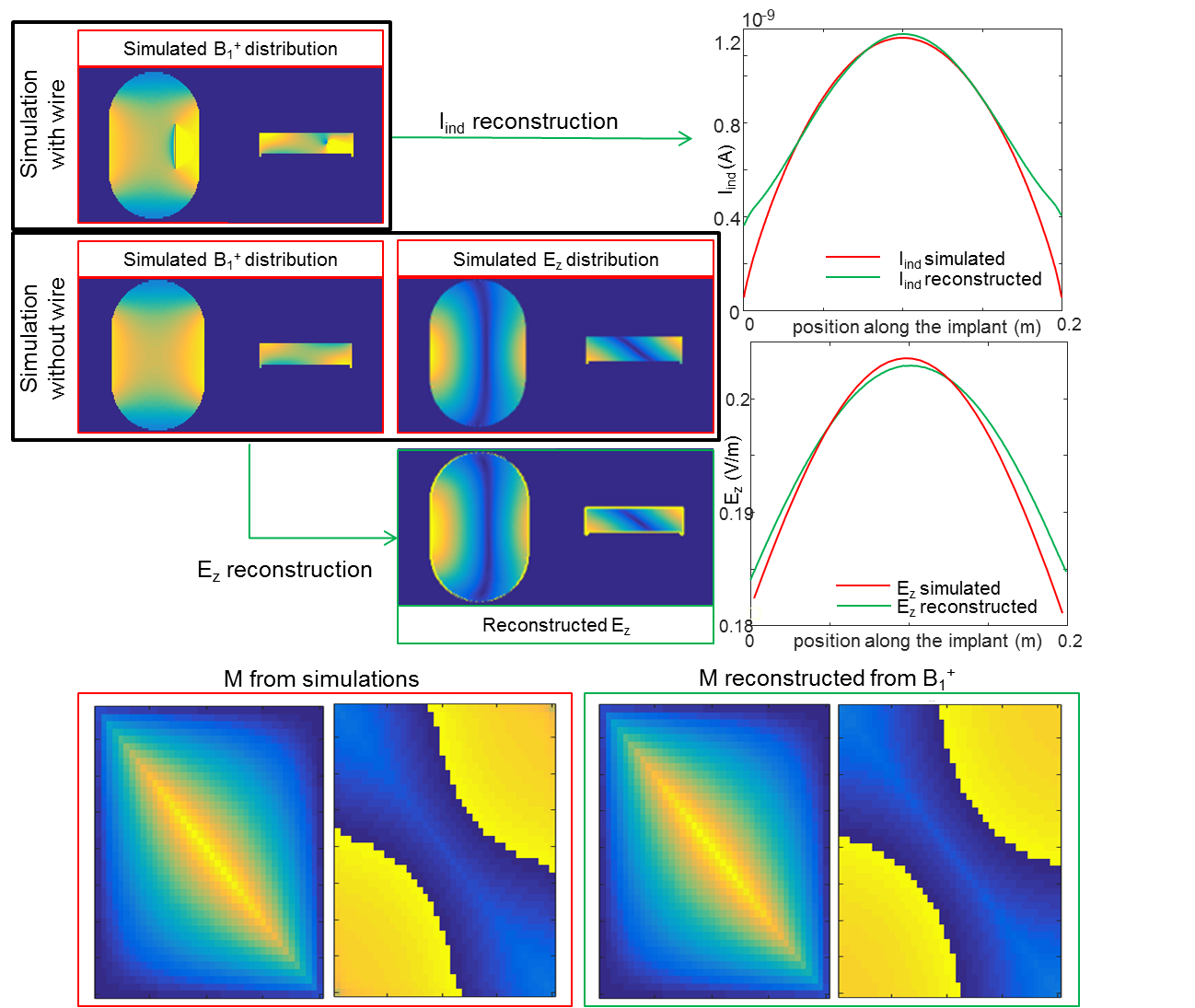
To demonstrate the feasibility of MRI-based assessment of the IRM, an MRI measurement is designed that was tested in silico: we simulated an MRI experiment of a large phantom, with $$$\sigma = 0.47S/m$$$ and $$$\epsilon_r=78$$$, with and without an implant present. The simulated B₁⁺ distribution without the implant, which is accessible from MRI acquisitions⁵ assuming the transceive phase approximaton⁶ to be valid, was used to determine $$$E_{inc}$$$ using the method from Buchenau et al⁷.

In a separate simulation with the implant in situ $$$I_{ind}$$$ is determined from the distortion in the B₁⁺ field⁸. $$$M$$$ is subsequently determined through:$$\tag{2}\underset{\vec{c}}{\text{min}}\|M(z_i,z_j;\vec{c})E_{inc}-I_{ind}\|,$$

where $$$\vec{c}\,$$$is the set of parameters,$$$\{\sigma_{eff}E_0,r_0,r_L,c_1,c_2,...,t_{12},t_{23},..\}$$$ describing the implant.

Results

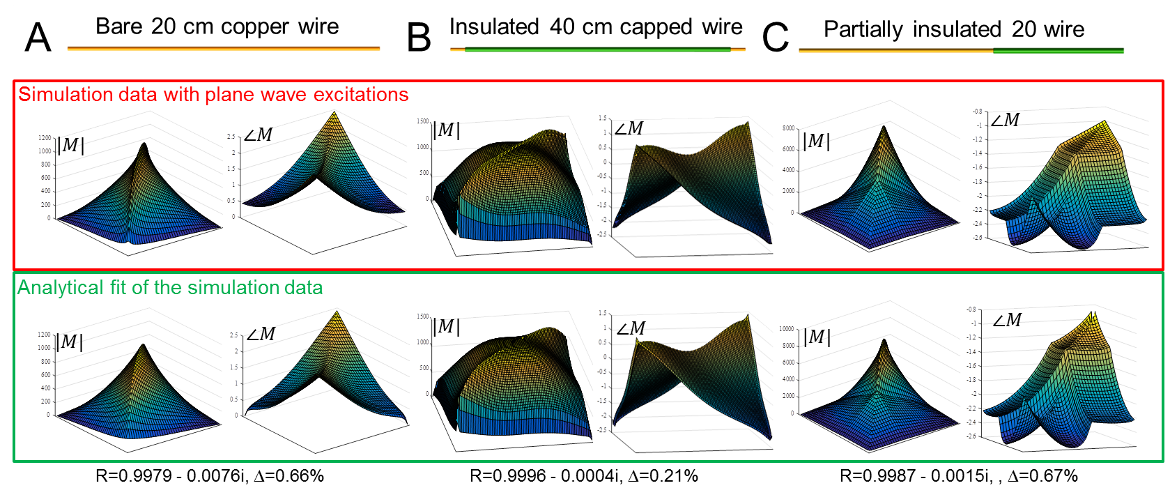
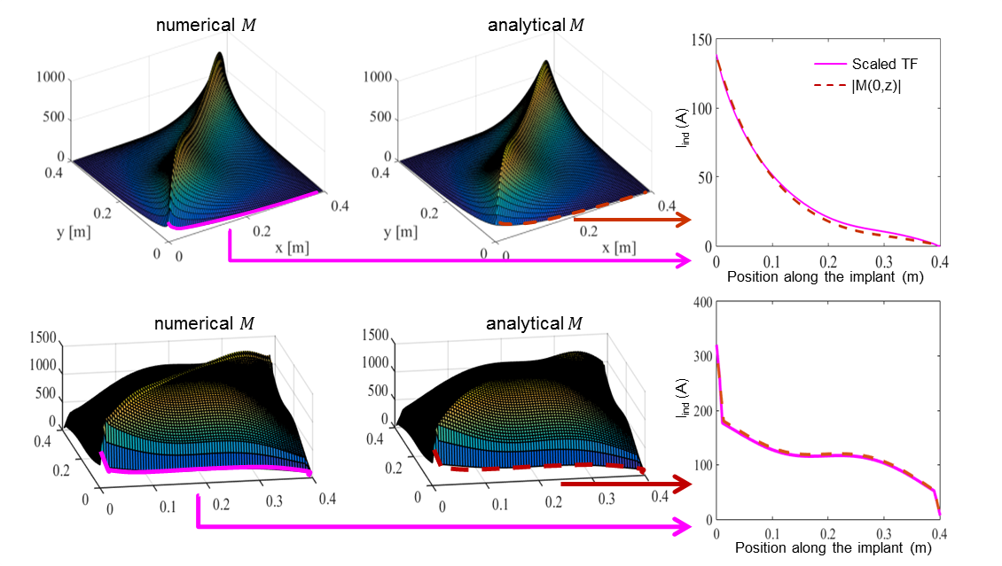
Both the simulated IRM (considered as ground truth) and the analytical fits using formula (1) are shown in figure 3. These are in good agreement (Pearson correlation coefficient $$$R:0.9979-0.9996$$$). This demonstrates the validity of expression (1). In figure 4 it is shown that the TFs are directly proportional to the first column of .

The feasibility of MRI based IRM determination is shown in figure 5. With merely B₁⁺ distributions from simulations with and without the implant the IRM was accurately reconstructed ($$$R:0.974$$$).

Discussion and conclusion

The IRM is an extended version of the TF, which actually is its first column. The feasibility of MRI based measurement of the IRM/TF has been demonstrated in silica. The actual experimental evalution of the IRM will be explored in the near future.

The IRM has been presented to characterize an implant’s response to impinging electric fields. With a model of converging infinite sums of reflected and transmitted damped waves an accurate analytical description of the IRM is derived. The analytical description of the RF response of an implant makes TF determination with regular MRI experiments feasible.

Acknowledgements

References

1. S.M. Park, et al., "Calculation of MRI-induced heating of an implanted medical lead wire with an electric eld transfer function". JMRI, 2007.

2.ISO/TS 10974, International Standards Organization Technical Specication, "Requirements for the safety of magnetic resonance imaging for patients withan active implantable medical device", 2011.

3. S. Feng, et al., "A technique to evaluate MRI-Induced Electric Fields at the Ends of Practical Implanted Lead", IEEE, 2015.

4. Tokaya, et al., "Ultra-Fast MRI Based Transfer Function Determination for the Assessment of Implant Safety", ISMRM proc, 2016.

5. V.L. Yarnykh, "Actual flip-angle imaging in the pulsed steady state: a method for rapid three-dimensional mapping of the transmitted radiofrequency field", Magn Reson Med, 2007.

6. A.L. van Lier, et al., "B+1phase mapping at 7 T and its application for in vivo electrical conductivity mapping", Magn Reson Med, 2012.

7. S. Buchenau, et al., "Iterative separation of transmit and receive phase contributions and B1+-based estimation of the specific absorption rate for transmit arrays", Magn Reson Mater Phy, 2013

8. M. R. van den Bosch, et al., "New method to quantify RF induced currents inside conductive wires", Proc. Int. Soc. Mag. Reson., 2009