Synopsis

In order to visualize the concentration and distribution of magnetic nanoparticles in pre-clinical research of magnetic nanoparticles-based sentinel lymph node biopsy, Quantitative Susceptibility Mapping(QSM) is a promising quantification tool in MRI. However, the strong magnetic field generated by high concentrations of magnetic particles causes the failure of conventional B0 map used in QSM. A novel spin echo-based View Line sequence with radius basic function interpolation-based reconstruction method has been proposed to obtain the B0 map for high concentrations of magnetic nanoparticles. This method has been verified by MRI data and simulation data for a range of iron in Resovist from 41 ug to 654 ug. Comparison of the reconstructed field map and theoretical field map provides normalized root mean square of $$$0.085\pm 0.054$$$ for the line field map, and $$$0.065 \pm 0.024$$$ for the interpolated field map.

Background and Purpose

Sentinel lymph node biopsy (SLNB) is a technique that has been used since 1977¹ to determine whether cancer cells metastasized during tumor removal surgery. Recently, a promising method to identify the location of sentinel lymph node during the surgery with less impact to the body has emerged². This method is based on detecting the accumulation amount of superparamagnetic iron oxide nanoparticles (SPIONs) in the body after pre-operative injection. Techniques for quantifying SPIONs with MRI can benefit preclinical research such as optimizing the protocol of SLNB based on SPIONs.

Previous studies have developed methods quantify low concentrations of SPIONs with MRI, but not high concentrations of SPIONs. These include the relaxometry method to quantify low concentration Fein SPIONs with MRI (0.05 mg/ml³, 0.1 mg/mL⁴, 0.2 mg/mL⁵), and B0 map-based QSM to visualize and quantify low-concentration SPIONs⁶. However, the conventional gradient recall echo (GRE)-based field map⁷ suffers from uncancelled phase shifts which increase the void signal area around high-concentration SPIONs.

The purpose of this study is to obtain a B0 map of high concentrations of SPIONs that generate strong inhomogeneous fields for subsequent quantitative analysis.

Methods

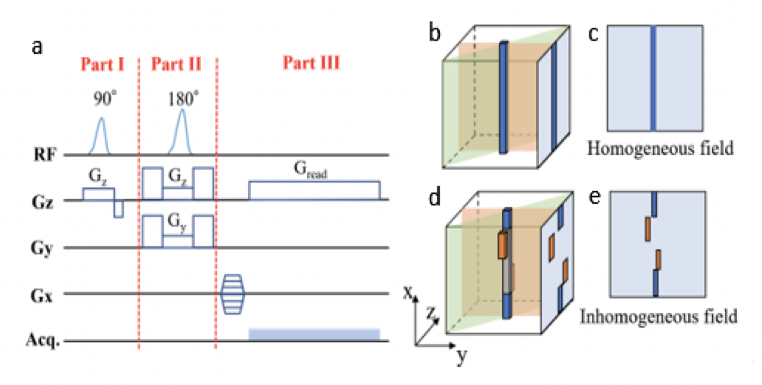
We propose a novel sequence called View Line modified from spin echo (SE) sequence to overcome the disadvantages of GRE. Unlike SEMAC⁸, this sequence does not encode slice distortion but extracts this distortion information and directly converts it into magnetic field strength.

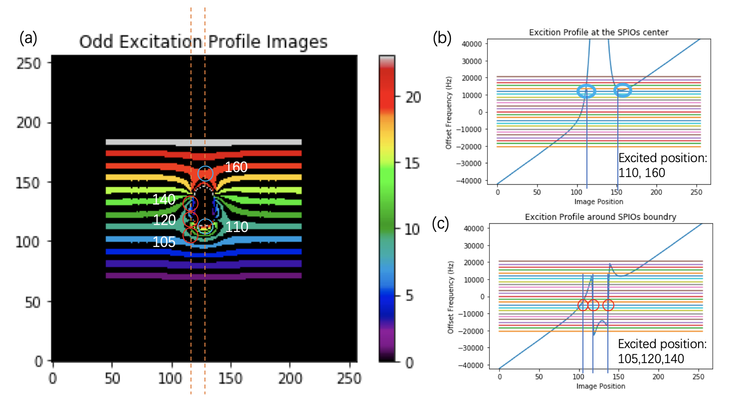
The sequence diagram is shown in Fig. 1. This method can be divided into three parts. Part I is the normal slice selection part and we can represent the actual excited inhomogeneous position ($$$z_0'$$$) with homogeneous position ($$$z_0$$$) as $$RF_{freq} \equiv \gamma G_z z_0 \equiv \gamma (G_z z_0' + \Delta B (x,y,z_0'))$$ $$z_0' = z_0 -\frac{\Delta B (x,y,z_0') }{G_z}$$, where $$$\gamma$$$ is the Larmor frequency, $$$G_z $$$ is the slice selection gradient, and $$$\Delta B (x,y,z_0')$$$ is the magnetic field at position $$$z_0'$$$. A more detailed excitation profile image is shown in Fig. 2, which visualizes this relationship. Part II achieves line selection, and part III is the readout module that includes frequency encoding and phase encoding. After the readout module, the excited spins with frequency encode gradient can be calculated as $$\omega (z_0) = \gamma G_{read} z_0 $$ $$ \omega (z_0' )=\gamma G_{read} z_0'+\gamma \Delta B (x,y,z_0') = \gamma G_{read} [z_0' + \frac{G_z(z_0-z_0')}{G_{read}}] $$. When represented in the MRI image, the spins in homogeneous position will have a signal at the correct position $$$z_0$$$ in the image. However, the spins excited in inhomogeneous position will locale at $$$z_0' + \frac{G_z(z_0-z_0')}{G_{read}}$$$ in the MRI image.

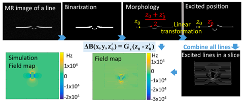
The goal of the reconstruction method is to reconstruct the field map from the warped MRI image. By setting $$$G_{read}$$$ to $$$2G_z$$$, the twisted region induced by the inhomogeneous magnetic field can be represented as $$$(z_0'+z_0 )/2 $$$. After the linear transfer, the excitation profile image can be obtained. This basic reconstruction method for extracting the line field map can also be seen as the preprocessing of the reconstruct, as shown in Fig. 3.

The next step in reconstruction is the use of the radius basis function (RBF) interpolation method, which is a real-valued function whose value depends only on the distance from the origin^9,10. In this work, we tested six forms of RBFs and evaluated the mean squared error of interpolated data to simulate the target data. Finally, the multiquadric function $$$\sqrt{1+(r/\epsilon)^2}$$$ was selected, and the shape parameter $$$\epsilon$$$ is 2 and 3 in the vertical and horizontal directions, respectively.

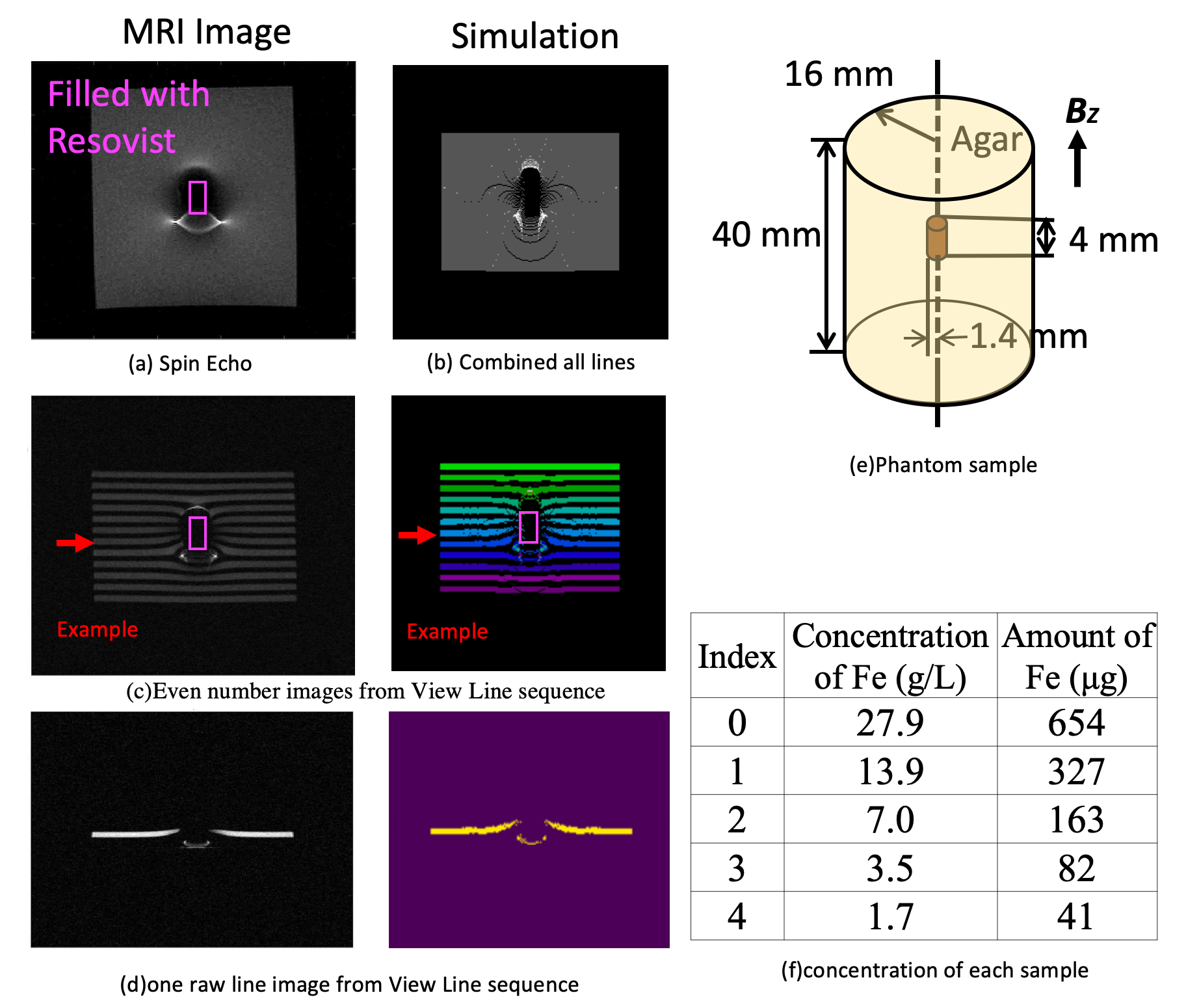
Verification Experiment

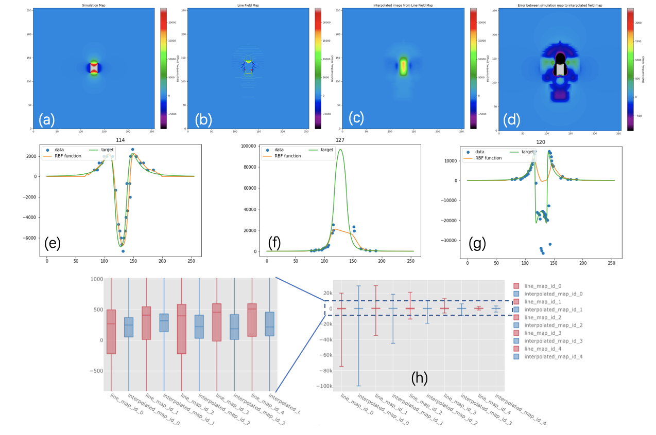
Verification experiments based on actual MRI data from 7T MRI (Bruker BioSpec) and artificial data (Python Program) were implemented. The experimental conditions and results are shown in Fig 4. Five different concentrations of magnetic particles were placed in the phantom. For the reconstruction algorithm, we compared the field map calculated from the magnetic moment¹¹ ($$$1.54*10^{-8} Am^2/ voxel, 1 voxel = 0.1953 mm^3$$$) and the field map reconstructed from the View Line sequence. The comparison results are shown in Fig. 5. The figure shows the reconstruction result of sample no. 2. The void signal area is unavoidable near the center after the RBF interpolation algorithm, but as shown in Fig. 5(c), there is a certain degree of mitigation. At the same time, Figs. 5(e–g) show the limitation of the algorithm, that is, the algorithm can restore the field map better away from the center, but it cannot restore the field map near the center owing to the void signal. The box plot statistics results are shown in Fig. 5(h). It can be seen that for five different concentrations of samples, the residual after interpolation processing is less than the line field map.

Acknowledgements

References

1. Cabanas, R. M. An approach for the treatment of penile carcinoma. Cancer39,456–466 (1977).

2. Sekino, M. et al.Handheld magnetic probe with permanent magnet and Hall sensor for identifying sentinel lymph nodes in breast cancer patients. Sci. Rep.8,1195 (2018).

3. Rad, A. M., Arbab, A. S., Jiang, Q. & Soltanian-zadeh, H. Quantification of Superparamagnetic Iron Oxide (SPIO)-labeled Cells Using MRI. 26,366–374 (2007).

4. Liu, W., Dahnke, H., Rahmer, J., Jordan, E. K. & Frank, J. A. Ultrashort T 2* relaxometry for quantitation of highly concentrated superparamagnetic iron oxide (SPIO) nanoparticle labeled cells. Magn. Reson. Med.61,761–766 (2009).

5. Pelot, N. A. & Bowen, C. V. Quantification of superparamagnetic iron oxide using inversion recovery balanced steady-state free precession. Magn. Reson. Imaging31,953–960 (2013).

6. Wong, R., Chen, X., Wang, Y., Hu, X. & Jin, M. M. Visualizing and quantifying acute inflammation using ICAM-1 specific nanoparticles and MRI quantitative susceptibility mapping. Ann. Biomed. Eng.40,1328–1338 (2012).

7. Bernstein, M. A., King, K. F. & Zhou, X. J. Handbook of MRI pulse sequences. (Academic Press, 2004).

8. Lu, W., Pauly, K. B., Gold, G. E., Pauly, J. M. & Hargreaves, B. a. SEMAC: Slice Encoding for Metal Artifact Correction in MRI. Magn. Reson. Med.62,66–76 (2009).

9. Fasshauer, G. E. Meshfree Approximation Methods with Matlab. 6,(WORLD SCIENTIFIC, 2007).

10. Schimek, M. G. Smoothing and Regression : Approaches, Computation, and Application.(Wiley, 2013).

11. Kuwahata, A. et al.Three-dimensional sensitivity mapping of a handheld magnetic probe for sentinel lymph node biopsy. AIP Adv.7,056720 (2017).