5058
Filter design for Breast Conductivity imaging Using phase-based gradient EPT (gEPT)1electrical electronic engineering, yonsei University, seoul, Korea, Republic of, 2Department of Radiology, Seoul National University Hospital, seoul, Korea, Republic of
Synopsis
EPT has a potential for immediate clinical use since it does not require additional hardware. However, there are various problems when applying
Introduction
EPT(Electrical Properties Tomography) is a non-invasive technique that extracts electrical properties from MR image1. This method has a potential for immediate clinical use since it does not require additional hardware. However, there are various problems when applying clinical practice. The B1 magnitude is hard to obtain due to time constraints, so phase-based method is often used2. Also, SNR of the B1 phase is of concern. Previously for breast conductivity studies, a reconstruction method based on magnitude-weighted polynomial fitting was proposed3. This method used kernelized fitting and magnitude weighting map to reduce boundary errors and noise amplification. However, if a large kernel is used or the ROI has a complex structure, this method creates erroneous conductivity images4. Recently, a new phase-based EPT technique called ‘gradient-based EPT’(pgEPT) was proposed5. This method reduces the boundary error by adding a gradient of phase term and reduce noise amplification by adding an artificial diffusion term. In this study, pgEPT for breast conductivity is proposed and filter design methods are explored for these terms.
Theory & Implementation
The pgEPT equation is shown in Eq 1.
$$$-c\cdot\triangledown^2\rho + \triangledown \phi^{tr} \triangledown \rho + \triangledown^2\phi^{tr}\rho = 2 \omega \mu_0$$$
(c is diffusion term constant, φtr is transceive phase, ρ is resistivity) (Eq. 1)
Eq 1. can be solved for using finite-difference method. Figure 1 shows conductivity reconstructed from conventional Helmholtz-EPT, magnitude-weighted polynomial fitting and pgEPT without dedicated filter specs [2]. Helmholtz-EPT has boundary-artifacts and noise amplification while magnitude-weighted polynomial fitting makes errors due to the sub-optimal large kernel size. pgEPT does not work properly due to the lack of SNR. Since the noise amplification of the Laplacian operation (3rd term in left side of Eq 1) is higher than gradient operation (2nd term in left side of Eq. 1), filtering the Laplacian of phase term should be stronger than the gradient of phase term. Therefore, it is not desirable to use large filtering kernel, and instead a second-order polynomial fitting was implemented for Laplacian operation (kernel size [5 5]).
Methods
1. Data Acquisition: experiments with a 3T clinical scanner (Skyra; Siemens Medical Solutions, Erlangen, Germany) A phantom with agarose: 12g/L, CuSO4:0.2g/L, NaCl:8g/L for inner cylinder and CuSO4:0.4g/L, NaCl:4g/L for background was used and the Turbo Spin echo (TSE) sequence with the following parameters was acquired: PDw 5mm thickness, image size=128×100, FOV=128×128mm, TR=4000ms, TEeff =10ms, ETL=5, number of slice=10. Averaging=4, Total scan time ~5.3min. For In-vivo breast imaging a TSE sequence with the following parameters was acquired: T2w 3.2-mm thickness, image size=384×260, FOV=320×320mm, TR=10800ms, TEeff =101ms, ETL=20, number of slice=45. Total scan time ~2.3 min.
2. EPT reconstruction: 1) conventional 2D-weighted polynomial fitting (kernel size=31x31), 2) pgEPT without filter optimization and 3) proposed method with dedicated filters were performed to reconstruct conductivity5.
Result
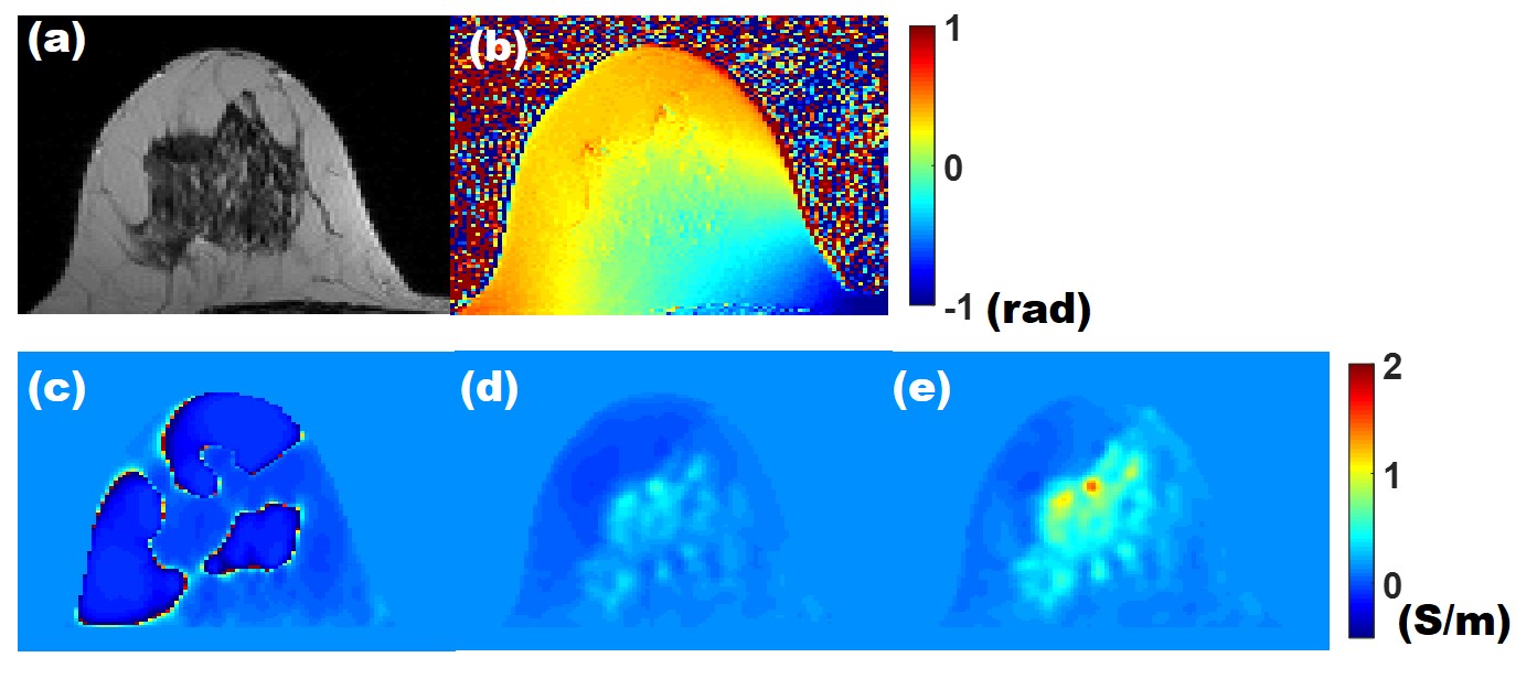
Figure 2 shows the effects of filtering on Laplacian and gradient of phase using the phantom data. Figure2.d shows the conductivity of the phantom. As shown in Figure 2b-c, the contrast of conductivity was removed after strong gaussian filtering on the gradient of phase, but the contrast of conductivity remained after strong gaussian filtering on Laplacian of phase. So, handling noise only using pre-filter is not a proper process. As shown in Figure 2 dedicated filter design is needed for each gradient and Laplacian term. Figure 3.a-b are in-vivo magnitude and phase of the T2-weighted image. Figure 3c-e show the results of polynomial fitting on the gradient of phase(Fig.3c), gradient and Laplacian of phase(Fig.3d) and Laplacian of phase only(Fig.3e). Without kernel fitting on Laplacian, conductivity result is unstable(Fig.3c) and with kernel fitting on the gradient of phase, the contrast of conductivity is reduced(Fig.3d). As shown in Figure3e, using the proposed method shows the stable and contrast-restored conductivity image. Figure 4 shows that the conductivity maps reconstructed by the conventional pgEPT and the proposed method with different strength of diffusion term and pre-filter. The conductivity map tends to be stabilized with increasing diffusion and pre-filter, but the contrast of conductivity is reduced. Finally, Figure 5 show in-vivo breast conductivity results. Arrows in figure 5.b indicate errors coming from large kernel size. Using the proposed approach (Fig.5c), conductivity value matched well with the parenchymal region in the magnitude of T2-weighted image with conductivity of higher than 0.3S/m.Discussion & Conclusion
Dealing with low SNR using filtering and regularization is necessary for conductivity imaging. The laplacian of phase term requires strong filtering in low SNR because of its high noise amplification. However, enlarging the spatial kernel should be avoided since it produces a blurred conductivity image. Here, polynomial fitting was implemented for strong noise reduction without enlarging the kernel. In this study, we did not handle the gradient of phase term which needs further investigation.Acknowledgements
No acknowledgement found.References
1. U. Katscher, T. Voigt, C. Findeklee, et al, Determination of Electric Conductivity and Local SAR Via B1 Mapping. IEEE TMI. 2009;28(9):1365-1374. 2.T. Voigt, Katscher U., Doessel O., Quantitative conductivity and permittivity imaging of the human brain using electrical properties tomography. Mag. Reson. Med., 2011;66(2): 456-466. 3. J Lee, Shin J., Kim DH., MR_Based Conductivity Imaging Using Multiple Receiver Coils. Magn Reson Med. 2016;76(2):530–539. 4. J. Kim, J. Shin, H. Lee, et al, Adaptive Weighted Polynomial fitting in Electrical Property Tomography (EPT). ISMRM 2017,#3643. 5. N. Gurler, Y. Z. Ider, Gradient-Based Electrical Conductivity Imaging Using MR Phase. Mag. Reson. Med., 2016;77(1):137-156.Figures