Synopsis

In this study, the recently proposed magnetic susceptibility source separation method, which separates the paramagnetic susceptibility source from the diamagnetic susceptibility source, was validated using Monte-Carlo simulation and phantom experiment. The results demonstrate that the method successfully separates the paramagnetic and diamagnetic susceptibility sources in both simulation and experiment.

Purpose

Methods

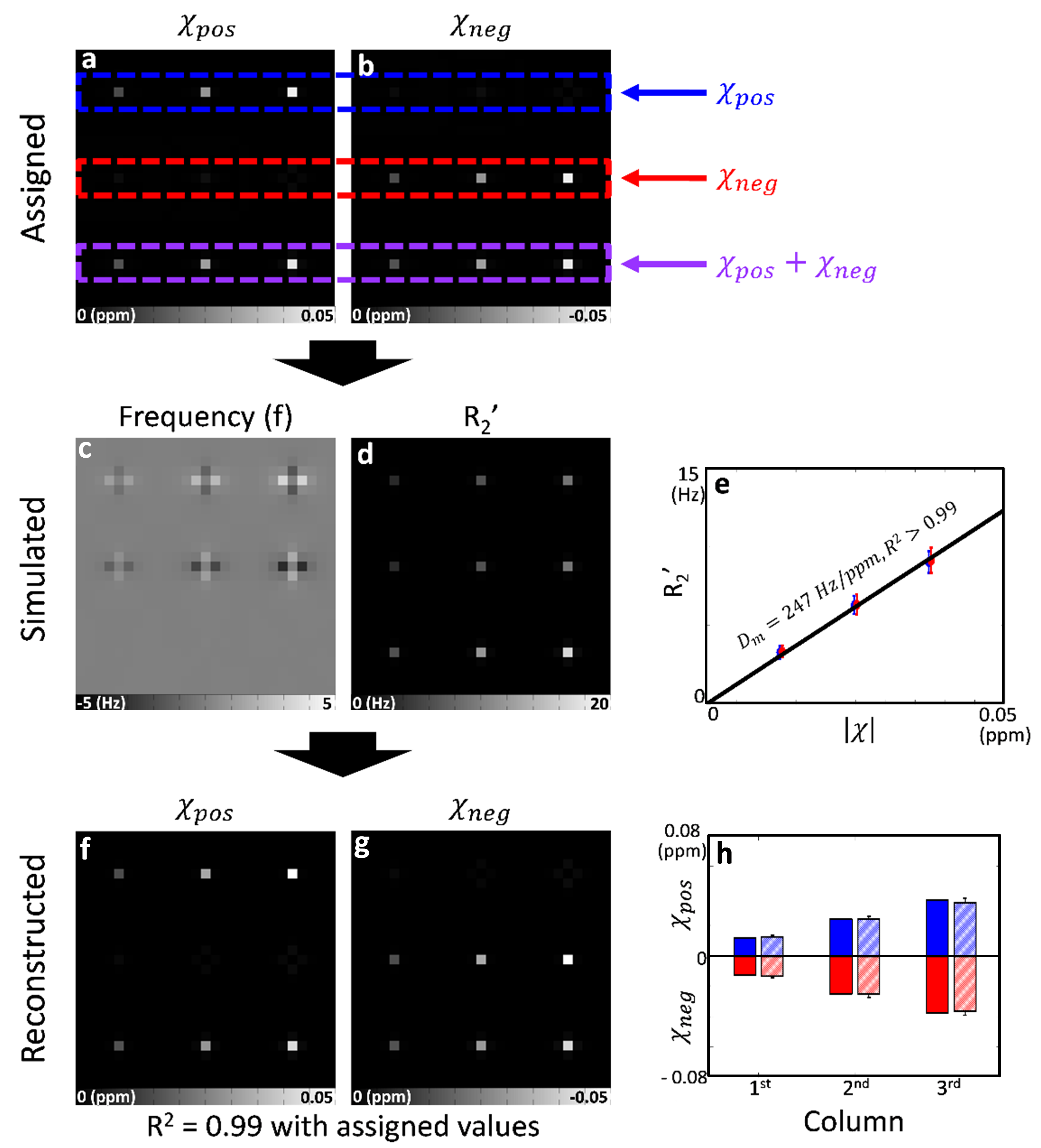
[Reconstruction algorithm] The positive and negative susceptibility maps ( and ) were reconstructed by solving the following equation (Fig. 1): $$argmin_{\chi_{pos}(r),\chi_{neg}(r)}\mid({R_2}'(r)+i2\pi f(r))-D_m\cdot(\mid\chi_{pos}(r)\mid+\mid\chi_{neg}(r)\mid)-i2\pi D_p(r)\otimes(\chi_{pos}(r)+\chi_{neg}(r))\mid_2+g(\chi_{pos}(r),\chi_{neg}(r))$$

where $$$D_m$$$ is a proportionality constant explaining for the effect size of susceptibility on R₂’, and $$$D_p$$$ is a dipole pattern². The $$$g(\chi_{pos}(r),\chi_{neg}(r))$$$ is an optional regularization term³.

[Monte-Carlo simulation] The nine simulation segments were designed to consider three susceptibility compositions (positive only, negative only, and half and half) and three source concentrations (|0.0125|, |0.025|, and |0.0375| ppm) (Fig. 1a-b). Each segment contained 9×9×9 voxels with a 100 µm size. Within a voxel, 1000 protons were randomly distributed by Gaussian diffusion model (1 µm²/ms). The susceptibility sources (diameter = 1 µm, susceptibility = |520| ppm) were randomly located within the central voxel. The voxel-averaged magnitude and phase were calculated from the sum of proton signals (T₂ = 100 ms). The R₂* decays and frequency shift were estimated using curve fitting. R₂’ was calculated as R₂* - R₂. All the simulation was repeated 100 times and averaged. The resulting data were processed using Eq. 1, generating the positive and negative susceptibility maps. $$$D_m$$$ was calculated from the slope of the simulated R₂’ values w.r.t. the assigned susceptibility values.

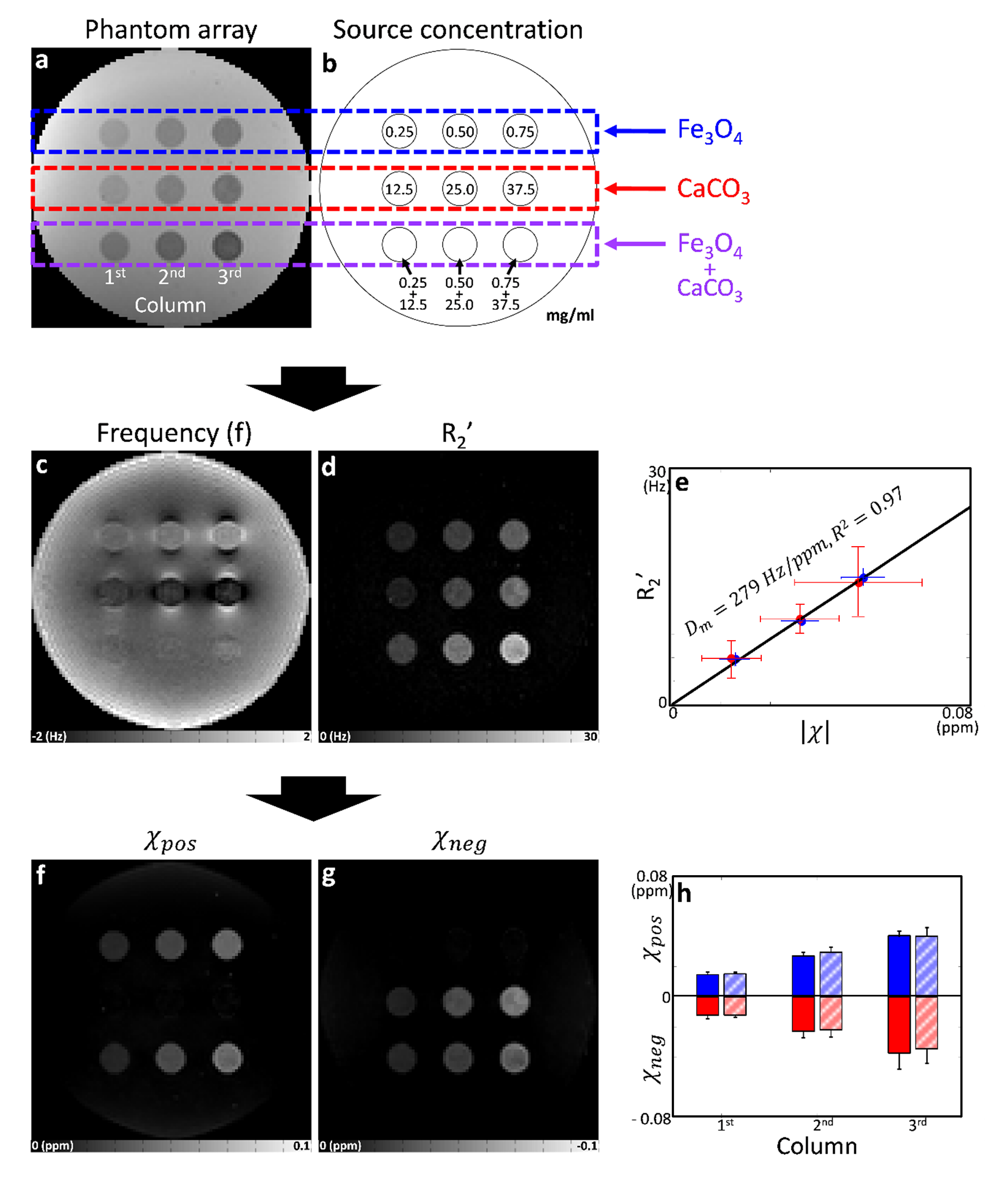
[phantom experiment] For phantom manufacturing, a cylindrical container (diameter = 120 mm) was constructed with nine small cylinders (diameter = 7 mm) (Fig. 2a). The medium was filled with 1.5% agarose gel. The nine small cylinders were filled with positive and/or negative susceptibility sources in agarose. For the positive and negative susceptibility sources, iron oxide (Fe₃O₄; 0.25, 0.50, 0.75 mg/ml; first row) and calcium carbonate (CaCO₃; 12.5, 25.0, and 37.5 mg/ml; second row) were used. The two sources were mixed for the third row with the same concentrations as the first two rows. For R₂* and frequency shift, multi-echo gradient-echo were acquired at 3T: FOV = 192×192×120 mm³, voxel size = 1×1×2 mm³, TR = 60 ms, and TE = 2.6:4.9:27.1 ms. For R₂ estimation, multi-echo spin-echo data were acquired: FOV = 192×192 mm², voxel size = 1×1 mm², slice thickness = 2 mm, number of slices = 40, TR = 4000 ms, and TE = 9:9:90 ms. The data were processed for R₂’ and frequency shift¹, and the source separation algorithm was applied to generate the positive and negative susceptibility maps. For $$$D_m$$$, the slope of R₂’ plot w.r.t. the absolute susceptibility values was calculated from the positive and negative only data.

Results

[Monte-Carlo simulation] The simulation setup is visualized in Fig. 2a-b. The simulated frequency shift maps show dipole patterns (Fig. 2c) whereas R₂’ shows localized signal change (Fig. 2d). The linear regression between R₂’ and susceptibility yields $$$D_m$$$ of 247 Hz/ppm (Fig. 2e). When the susceptibility source separation method is applied, the positive and negative susceptibility maps are reconstructed with high fidelity (R² = 0.99 with the assigned maps; Fig. 2f-g). The results shown in the bar graph reveal consistent measurements (Fig. 2h).

[phantom experiment] The phantom experimental results further corroborate our method. The phantom setup is shown in Figs. 3a-b. The frequency shift map shows dipole patterns around the susceptibility sources (Fig. 3c). On the other hand, R₂’ is dependent on the absolute sum of the susceptibility as shown in Fig. 3d. When the R₂’ values of the single sources are plotted w.r.t. the susceptibility (Fig. 3e; blue dots: Fe₃O₄ and red dots: CaCO₃), linear dependence is observed for both sources with the average $$$D_m$$$ of 279 Hz/ppm. When the sources are separated (Fig. 3f-g), they clearly show positive and negative susceptibility contributions exclusively. In the third row, the mixed sources are successfully separated, revealing the similar positive and negative susceptibility concentrations with the first and second rows (Fig. 3h). These results demonstrate that our method successfully separated positive and negative susceptibility sources with high accuracy.

Discussion and conclusion

Acknowledgements

References

[1] Lee, J., Nam, Y., Choi, J.Y., Shin, H.G., Hwang, T., Lee, J., 2017. Separating positive and negative susceptibility sources in QSM. Proc Intl Soc Mag Reson Med 25, 0751.[2] Salomir, R., de Senneville, B.D., Moonen, C.T.W., 2003. A fast calculation method for magnetic field inhomogeneity due to an arbitrary distribution of bulk susceptibility. Concepts in Magnetic Resonance Part B: Magnetic Resonance Engineering 19B, 26-34.[3] Liu, T., Liu, J., de Rochefort, L., Spincemaille, P., Khalidov, I., Ledoux, J.R., Wang, Y., 2011. Morphology enabled dipole inversion (MEDI) from a single-angle acquisition: comparison with COSMOS in human brain imaging. Magn Reson Med 66, 777-783.